In this page, we discuss how to calculate the distance between planes, lines, points, and everything in between. We will show why the distance formula is such, but once the formula is concluded, you are not expected to repeat the work but rather use the formula.
It should be clear at this point, that given two points  and
and  , the distance between them is the magnitude of the vector connecting them, that is:
  .
.
Distance Between a Point and a Line
Theorem 9.1 (Distance Between a Point and a Line): Let  be a point in
  and
and  a line with initial point and direction vector
  . The shortest distance
  from the point to the line is given by the ratio of the magnitude of their vector cross product to the magnitude of the direction vector.
![\[d(M, \ell) = \frac{\|\overrightarrow{AM} \times \vec{u}\|}{\|\vec{u}\|}\]](https://mathematics.lu/wp-content/ql-cache/quicklatex.com-ab44aa10a4aff12e36b4d738300006c0_l3.png "Rendered by QuickLaTeX.com")
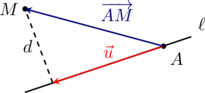
![\[\text{Area} = \frac{1}{2} \|\vec{u} \times \overrightarrow{AM}\|\]](https://mathematics.lu/wp-content/ql-cache/quicklatex.com-1ea672d4744dc5d6ba2a5f1ca59a6046_l3.png "Rendered by QuickLaTeX.com")
![\[\text{Area} = \frac{1}{2} \cdot d \cdot \|\vec{u}\|\]](https://mathematics.lu/wp-content/ql-cache/quicklatex.com-2dd888999defb1448e11d83f683e7452_l3.png "Rendered by QuickLaTeX.com")
![\[\frac{1}{2} \cdot d \cdot \|\vec{u}\| = \frac{1}{2} \|\vec{u} \times \overrightarrow{AM}\| \implies d = \frac{\|\vec{u} \times \overrightarrow{AM}\|}{\|\vec{u}\|}\]](https://mathematics.lu/wp-content/ql-cache/quicklatex.com-c8ae275f2341038371cbae3d35efc621_l3.png "Rendered by QuickLaTeX.com")
In the formula above, is any point belong to the line.
Example: Calculate the shortest distance from the point  to the line given by the parametric equations:
![\[\ell: \begin{cases} x = 1 + 2t \\ y = -1 - t \\ z = 2 + 2t \end{cases}\]](https://mathematics.lu/wp-content/ql-cache/quicklatex.com-1780084999a472192107a9c16e4b9f29_l3.png "Rendered by QuickLaTeX.com")
![\[A(1, -1, 2), \quad \vec{u} = \begin{pmatrix} 2 \\ -1 \\ 2 \end{pmatrix}\]](https://mathematics.lu/wp-content/ql-cache/quicklatex.com-14bae31fd2482230ede9d1b709cac244_l3.png "Rendered by QuickLaTeX.com")

![\[\overrightarrow{AM} = \begin{pmatrix} 2 - 1 \\ 1 - (-1) \\ 3 - 2 \end{pmatrix} = \begin{pmatrix} 1 \\ 2 \\ 1 \end{pmatrix}\]](https://mathematics.lu/wp-content/ql-cache/quicklatex.com-de142a9a391e2ccc3c94d3a0d21ca90a_l3.png "Rendered by QuickLaTeX.com")

![\[\overrightarrow{AM} \times \vec{u} = \begin{pmatrix} (2)(2) - (1)(-1) \\ (1)(2) - (1)(2) \\ (1)(-1) - (2)(2) \end{pmatrix} = \begin{pmatrix} 4 + 1 \\ 2 - 2 \\ -1 - 4 \end{pmatrix} = \begin{pmatrix} 5 \\ 0 \\ -5 \end{pmatrix}\]](https://mathematics.lu/wp-content/ql-cache/quicklatex.com-11e378d5c701ee56283264ca5350b20d_l3.png "Rendered by QuickLaTeX.com")
![\[\|\overrightarrow{AM} \times \vec{u}\| = \sqrt{5^2 + 0^2 + (-5)^2} = \sqrt{25 + 0 + 25} = \sqrt{50} = 5\sqrt{2}\]](https://mathematics.lu/wp-content/ql-cache/quicklatex.com-745e8a2d28e205a324734dab44f18737_l3.png "Rendered by QuickLaTeX.com")
![\[\|\vec{u}\| = \sqrt{2^2 + (-1)^2 + 2^2} = \sqrt{4 + 1 + 4} = \sqrt{9} = 3\]](https://mathematics.lu/wp-content/ql-cache/quicklatex.com-bc51d9620037fdd5d4bb28d4fba77966_l3.png "Rendered by QuickLaTeX.com")
![\[d(M, \ell) = \frac{\|\overrightarrow{AM} \times \vec{u}\|}{\|\vec{u}\|} = \frac{5\sqrt{2}}{3}\]](https://mathematics.lu/wp-content/ql-cache/quicklatex.com-2bf26add2cf52e972070bc2ec47c3a5a_l3.png "Rendered by QuickLaTeX.com")
Distance Between Parallel Lines
If two lines are parallel, pick a point on any one line, and use the formula above to calculate the distance from that point to the other line.
Example: Calculate the distance between the two parallel lines  and
and  given by:
![\[\ell_1: \begin{cases} x = 1 + t \\ y = 2t \\ z = -1 - t \end{cases} \quad \text{and} \quad \ell_2: \begin{cases} x = 2 + s \\ y = 2 + 2s \\ z = 1 - s \end{cases}\]](https://mathematics.lu/wp-content/ql-cache/quicklatex.com-963689371342d17f1f7b2562fae98582_l3.png "Rendered by QuickLaTeX.com")
 to pick a reference point
 ![\[P(1, 0, -1)\]](https://mathematics.lu/wp-content/ql-cache/quicklatex.com-557121ebd38d204a44af514b90a26cde_l3.png "Rendered by QuickLaTeX.com")
![\[A(2, 2, 1), \quad \vec{u} = \begin{pmatrix} 1 \\ 2 \\ -1 \end{pmatrix}\]](https://mathematics.lu/wp-content/ql-cache/quicklatex.com-fcd3a570a6aa248b069ebf9c111fbfeb_l3.png "Rendered by QuickLaTeX.com")

![\[\overrightarrow{AP} = \begin{pmatrix} 1 - 2 \\ 0 - 2 \\ -1 - 1 \end{pmatrix} = \begin{pmatrix} -1 \\ -2 \\ -2 \end{pmatrix}\]](https://mathematics.lu/wp-content/ql-cache/quicklatex.com-f7ec94ff9fa2bcf7951ff349e66f7276_l3.png "Rendered by QuickLaTeX.com")

![\[\overrightarrow{AP} \times \vec{u} = \begin{pmatrix} (-2)(-1) - (-2)(2) \\ (-2)(1) - (-1)(-1) \\ (-1)(2) - (-2)(1) \end{pmatrix} = \begin{pmatrix} 2 + 4 \\ -2 - 1 \\ -2 + 2\end{pmatrix} = \begin{pmatrix} 6 \\ -3 \\ 0 \end{pmatrix}\]](https://mathematics.lu/wp-content/ql-cache/quicklatex.com-36b426efb1e78cac613a8952513a337c_l3.png "Rendered by QuickLaTeX.com")
![\[\|\overrightarrow{AP} \times \vec{u}\| = \sqrt{6^2 + (-3)^2 + 0^2} = \sqrt{36 + 9 + 0} = \sqrt{45} = 3\sqrt{5}\]](https://mathematics.lu/wp-content/ql-cache/quicklatex.com-bce48b40df3d01ab8c3d7c90db218ff1_l3.png "Rendered by QuickLaTeX.com")
![\[\|\vec{u}\| = \sqrt{1^2 + 2^2 + (-1)^2} = \sqrt{1 + 4 + 1} = \sqrt{6}\]](https://mathematics.lu/wp-content/ql-cache/quicklatex.com-aa37d4e13b51b17fe382ac6c494f22fd_l3.png "Rendered by QuickLaTeX.com")
![\[d(\ell_1, \ell_2) = \frac{\|\overrightarrow{AP} \times \vec{u}\|}{\|\vec{u}\|} = \frac{3\sqrt{5}}{\sqrt{6}} = \frac{3\sqrt{30}}{6} = \frac{\sqrt{30}}{2}\]](https://mathematics.lu/wp-content/ql-cache/quicklatex.com-e96808679cfde184b393547515c60709_l3.png "Rendered by QuickLaTeX.com")
Distance Between a Point and a Plane
Theorem 9.2: Let  be a point in and
  a plane. The distance between them is given by:
![\[d(M,\pi) = \frac{|a \cdot x_1 + b \cdot y_1 + c \cdot z_1 + d|}{\sqrt{a^2 + b^2 + c^2}}\]](https://mathematics.lu/wp-content/ql-cache/quicklatex.com-b72b38b8a00cd5d1159ca52c4a51d7dc_l3.png "Rendered by QuickLaTeX.com")
 the desired distance. Consider the following diagram: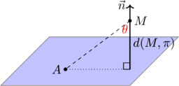
 . This is:
![\[\cos(\theta) = \frac{d(M,\pi)}{\|\overrightarrow{AM}\|} \implies d(M,\pi) = \cos(\theta) \cdot \|\overrightarrow{AM}\|\]](https://mathematics.lu/wp-content/ql-cache/quicklatex.com-7ea9b04480fc0ca5776d212aec4c31f8_l3.png "Rendered by QuickLaTeX.com")
 by its formula:
![\[d(M,\pi) = \frac{|\langle\overrightarrow{AM}, \vec{n}\rangle|}{\|\overrightarrow{AM}\| \cdot \|\vec{n}\|} \cdot \|\overrightarrow{AM}\| = \frac{|\langle\overrightarrow{AM}, \vec{n}\rangle|}{\|\vec{n}\|} = \frac{|a \cdot x_1 + b \cdot y_1 + c \cdot z_1 + d|}{\sqrt{a^2 + b^2 + c^2}}\]](https://mathematics.lu/wp-content/ql-cache/quicklatex.com-7f372040e4f9d5e4a1c6047f6e1b08a3_l3.png "Rendered by QuickLaTeX.com")
 . Then:
![\[\overrightarrow{AM} = \begin{pmatrix} x_1 - x_2 \\ y_1 - y_2 \\ z_1 - z_2 \end{pmatrix}\]](https://mathematics.lu/wp-content/ql-cache/quicklatex.com-a7d71b227de60b7cc6ac58e725ba3fae_l3.png "Rendered by QuickLaTeX.com")
![\[\langle\overrightarrow{AM}, \vec{n}\rangle = (x_1 - x_2) \cdot a + (y_1 - y_2) \cdot b + (z_1 - z_2) \cdot c\]](https://mathematics.lu/wp-content/ql-cache/quicklatex.com-287385a2cac9cbbf71bf96ffc3f9d5ef_l3.png "Rendered by QuickLaTeX.com")
![\[= a \cdot x_1 + b \cdot y_1 + c \cdot z_1 + \underbrace{(-a \cdot x_2 - b \cdot y_2 - c \cdot z_2)}_{d}\]](https://mathematics.lu/wp-content/ql-cache/quicklatex.com-2c04e2ea5b4c2b9a6760f8c847da69bb_l3.png "Rendered by QuickLaTeX.com")
Example: Calculate the shortest distance  from the point
  to the plane
  defined by the Cartesian equation
  .
.
 and the coefficients
  from the lowercase Cartesian equation:
![\[(x_1, y_1, z_1) = (1, 3, -2)\]](https://mathematics.lu/wp-content/ql-cache/quicklatex.com-4295896ce8c846d44be99d19727dfdd0_l3.png "Rendered by QuickLaTeX.com")
![\[a = 3, \quad b = -2, \quad c = 6, \quad d = -5\]](https://mathematics.lu/wp-content/ql-cache/quicklatex.com-3ed6cab121ec1025f97fee7e20a59551_l3.png "Rendered by QuickLaTeX.com")
![\[D = \frac{|a \cdot x_1 + b \cdot y_1 + c \cdot z_1 + d|}{\sqrt{a^2 + b^2 + c^2}}\]](https://mathematics.lu/wp-content/ql-cache/quicklatex.com-392fbda5c48aafe8c4f1716e7a2145d3_l3.png "Rendered by QuickLaTeX.com")
![\[D = \frac{|3(1) + (-2)(3) + 6(-2) - 5|}{\sqrt{3^2 + (-2)^2 + 6^2}}\]](https://mathematics.lu/wp-content/ql-cache/quicklatex.com-116124c5edd2f347e5993b596a11606c_l3.png "Rendered by QuickLaTeX.com")
![\[D = \frac{|3 - 6 - 12 - 5|}{\sqrt{9 + 4 + 36}} = \frac{|-20|}{\sqrt{49}} = \frac{20}{7}\]](https://mathematics.lu/wp-content/ql-cache/quicklatex.com-0d3b4583484e892163009cc1bc162754_l3.png "Rendered by QuickLaTeX.com")
Distance Between Two Parallel Planes
As before, if two planes are parallel, pick a point belong to one of the planes and use the formula above to find the distance between that point and the other plane.
Example: Calculate the distance between the two parallel planes  and
and  given by their Cartesian equations:
![\[\pi_1: 2x - y + 2z - 4 = 0 \quad \text{and} \quad \pi_2: 2x - y + 2z + 5 = 0\]](https://mathematics.lu/wp-content/ql-cache/quicklatex.com-002d3516867e2c4739c7797ae644737a_l3.png "Rendered by QuickLaTeX.com")
 and
and  :
:![\[2x - (0) + 2(0) - 4 = 0 \implies 2x = 4 \implies x = 2\]](https://mathematics.lu/wp-content/ql-cache/quicklatex.com-d37b46ab577234baf62a794ddb421771_l3.png "Rendered by QuickLaTeX.com")
 that lies directly on plane
  ,
,  ,
,  , and the constant
 ![\[a = 2, \quad b = -1, \quad c = 2, \quad d = 5\]](https://mathematics.lu/wp-content/ql-cache/quicklatex.com-cb2027ec9b4b03bcaff3b586ae77fd55_l3.png "Rendered by QuickLaTeX.com")
![\[D = \frac{|2(2) + (-1)(0) + 2(0) + 5|}{\sqrt{2^2 + (-1)^2 + 2^2}}\]](https://mathematics.lu/wp-content/ql-cache/quicklatex.com-f9ec15828373cb11a3e560c916cc24a6_l3.png "Rendered by QuickLaTeX.com")
![\[D = \frac{|4 + 0 + 0 + 5|}{\sqrt{4 + 1 + 4}} = \frac{9}{\sqrt{9}} = \frac{9}{3} = 3\]](https://mathematics.lu/wp-content/ql-cache/quicklatex.com-e12afefc7d6f87547028ea4a9c4153ec_l3.png "Rendered by QuickLaTeX.com")
Distance Between Skew Lines
To find the distance between skew lines, we need to find the points on the lines that are closest to one another. In order to do that, we take general points on each line (using each equation of the line), and create a generic vector  . Since will represent the distance, it needs to be perpendicular to both and . Therefore, the scalar product with the direction vectors of both lines must be 0. Since will depend on the parameters of the lines, and each scalar product yields an equation, this will give two equations with two variables. Finding the parameters, we can replace them to conclude , , and from which we conclude the distance.
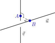
Alternatively, we can argue that this double perpendicularity condition can be used as:
![\[\vec{AB}=k\cdot\|\vec{u}\times\vec{v}\|\]](https://mathematics.lu/wp-content/ql-cache/quicklatex.com-0e7277ec78526150818d95edd9544609_l3.png "Rendered by QuickLaTeX.com")
We will see examples using both methods and then conclude the formula.
Example: Find the distance between the skew lines given in vector form by analyzing the perpendicular properties of their shortest connecting segment:
![\[\ell_1: \begin{pmatrix} x \\ y \\ z \end{pmatrix} = \begin{pmatrix} 0 \\ 1 \\ 2 \end{pmatrix} + t\begin{pmatrix} 1 \\ -1 \\ 1 \end{pmatrix} \quad \text{and} \quad \ell_2: \begin{pmatrix} x \\ y \\ z \end{pmatrix} = \begin{pmatrix} 3 \\ -1 \\ 4 \end{pmatrix} + s\begin{pmatrix} -1 \\ 2 \\ -1 \end{pmatrix} \quad \text{with } s, t \in \mathbb{R}\]](https://mathematics.lu/wp-content/ql-cache/quicklatex.com-87ef714f6e7a956f452d4a065be8e70e_l3.png "Rendered by QuickLaTeX.com")

![\[A(t, 1 - t, 2 + t), \quad B(3 - s, -1 + 2s, 4 - s)\]](https://mathematics.lu/wp-content/ql-cache/quicklatex.com-7c9048c4d7f8486894499d02e83e8087_l3.png "Rendered by QuickLaTeX.com")
![\[\overrightarrow{AB} = \begin{pmatrix} 3 - s - t \\ -2 + 2s + t \\ 2 - s - t \end{pmatrix}\]](https://mathematics.lu/wp-content/ql-cache/quicklatex.com-86f9dde643099a4a4c446adacd1a8d8f_l3.png "Rendered by QuickLaTeX.com")
 and
and  :
:![\[\begin{cases} \overrightarrow{AB} \cdot \vec{u} = 0 \implies (3 - s - t)(1) + (-2 + 2s + t)(-1) + (2 - s - t)(1) = 0 \\ \overrightarrow{AB} \cdot \vec{v} = 0 \implies (3 - s - t)(-1) + (-2 + 2s + t)(2) + (2 - s - t)(-1) = 0 \end{cases}\]](https://mathematics.lu/wp-content/ql-cache/quicklatex.com-59106791e166c07d06b7ab4425182a34_l3.png "Rendered by QuickLaTeX.com")
 and
and  :
:![\[\begin{cases} 3 - s - t + 2 - 2s - t + 2 - s - t = 0 \implies -4s - 3t = -7 \quad \text{(Eq. 1)} \\ -3 + s + t - 4 + 4s + 2t - 2 + s + t = 0 \implies 6s + 4t = 9 \quad \text{(Eq. 2)} \end{cases}\]](https://mathematics.lu/wp-content/ql-cache/quicklatex.com-afbb76abbff202e095454204c476bfa6_l3.png "Rendered by QuickLaTeX.com")
 and Equation 2 by
  , then add them together to eliminate
 ![\[4(-4s - 3t) + 3(6s + 4t) = 4(-7) + 3(9)\]](https://mathematics.lu/wp-content/ql-cache/quicklatex.com-5bd3590b633a004be3cbdf91b0d2c48f_l3.png "Rendered by QuickLaTeX.com")
![\[-16s - 12t + 18s + 12t = -28 + 27 \implies 2s = -1 \implies s = -0.5\]](https://mathematics.lu/wp-content/ql-cache/quicklatex.com-97b9babab3ce3eeefb1a5fc52ce601b8_l3.png "Rendered by QuickLaTeX.com")
 back into Equation 1 to find the value of
 ![\[-4(-0.5) - 3t = -7 \implies 2 - 3t = -7 \implies -3t = -9 \implies t = 3\]](https://mathematics.lu/wp-content/ql-cache/quicklatex.com-33cab3047661fca042ace147491b30c6_l3.png "Rendered by QuickLaTeX.com")
 and
and ![\[A = (3, -2, 5)\]](https://mathematics.lu/wp-content/ql-cache/quicklatex.com-7a9502d80de1b06deaf97aec11258df0_l3.png "Rendered by QuickLaTeX.com")
![\[B = (3.5, -2, 4.5)\]](https://mathematics.lu/wp-content/ql-cache/quicklatex.com-d2d1a455141aaeaef34e5c352c31512e_l3.png "Rendered by QuickLaTeX.com")
![\[\overrightarrow{AB} = \begin{pmatrix} 3.5 - 3 \\ -2 - (-2) \\ 4.5 - 5 \end{pmatrix} = \begin{pmatrix} 0.5 \\ 0 \\ -0.5 \end{pmatrix}\]](https://mathematics.lu/wp-content/ql-cache/quicklatex.com-027c0a745408bb03e4320ea19292e4dc_l3.png "Rendered by QuickLaTeX.com")
![\[\|\overrightarrow{AB}\| = \sqrt{(0.5)^2 + 0^2 + (-0.5)^2} = \sqrt{0.25 + 0 + 0.25} = \sqrt{0.5} = \frac{1}{\sqrt{2}}\]](https://mathematics.lu/wp-content/ql-cache/quicklatex.com-c85d21aff3cee97e7b2a72f78a4a2530_l3.png "Rendered by QuickLaTeX.com")
Example: Find the distance between the skew lines given in vector form by:
 and a point
  .
.![\[\overrightarrow{AB} = \begin{pmatrix} 3 - s - t \\ -1 + 2s - (1 - t) \\ 4 - s - (2 + t) \end{pmatrix} = \begin{pmatrix} 3 - s - t \\ -2 + 2s + t \\ 2 - s - t \end{pmatrix}\]](https://mathematics.lu/wp-content/ql-cache/quicklatex.com-5bbd67f92ff24eef52e7563dd171bc71_l3.png "Rendered by QuickLaTeX.com")
![\[\vec{v} = \begin{pmatrix} 1 \\ -1 \\ 1 \end{pmatrix} \quad \text{and} \quad \vec{w} = \begin{pmatrix} -1 \\ 2 \\ -1 \end{pmatrix}\]](https://mathematics.lu/wp-content/ql-cache/quicklatex.com-749da241e3f5eb031d00f844aa521a19_l3.png "Rendered by QuickLaTeX.com")
![\[\vec{v} \times \vec{w} = \begin{pmatrix} (-1)(-1) - (1)(2) \\ (1)(-1) - (1)(-1) \\ (1)(2) - (-1)(-1) \end{pmatrix} = \begin{pmatrix} -1 \\ 0 \\ 1 \end{pmatrix}\]](https://mathematics.lu/wp-content/ql-cache/quicklatex.com-a094e05492d579f3554fae0987b25958_l3.png "Rendered by QuickLaTeX.com")
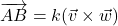 ) to create our linear system as follows:
![\[\begin{cases} 3 - s - t = -k \\ -2 + 2s + t = 0 \\ 2 - s - t = k \end{cases}\]](https://mathematics.lu/wp-content/ql-cache/quicklatex.com-d12e969eedc18076b87f318388403126_l3.png "Rendered by QuickLaTeX.com")
 or to find
 ![\[1 = -2k \implies k = -0.5 \implies \overrightarrow{AB} = \begin{pmatrix} 0.5 \\ 0 \\ -0.5 \end{pmatrix}\]](https://mathematics.lu/wp-content/ql-cache/quicklatex.com-68a632c04db918a6e9e43adc7739b995_l3.png "Rendered by QuickLaTeX.com")
![\[\|\overrightarrow{AB}\| = \sqrt{(0.5)^2 + 0^2 + (-0.5)^2} = \frac{1}{\sqrt{2}}\]](https://mathematics.lu/wp-content/ql-cache/quicklatex.com-bfe338b602206d18ffd22b3e4628c8be_l3.png "Rendered by QuickLaTeX.com")
Theorem (Distance Between Two Skew Lines): Let and be two skew lines in three-dimensional space . Let  be a fixed point on with direction vector
  , and let
  be a fixed point on with direction vector . The distance
  between the two lines is given:
![\[d(\ell_1, \ell_2) = \frac{|\overrightarrow{A_1A_2} \cdot (\vec{v} \times \vec{u})|}{\|\vec{v} \times \vec{u}\|}\]](https://mathematics.lu/wp-content/ql-cache/quicklatex.com-eda01b9f5c2e028433946d19a5a3f71f_l3.png "Rendered by QuickLaTeX.com")
The numerator in this formula is called the scalar triple product and represents the volume of a parallelepiped created by those vectors (we will see this later). Divided by the area of the basis, that gives the “height” which in this case is the distance between the lines. Just a way to think about where the formula comes from and why you can use any points that you want.
Finally, note that we cannot use this formula for parallel lines because the vector product would not be defined if the two vectors were parallel.
Exercises
For each problem below, find the shortest distance from the given point to the line in .
- 1. Point
 and line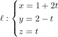
- 2. Point
 and line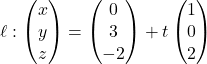
- 3. Point
 and line
Analyze each pair of lines below to determine their geometric relationship, then calculate the shortest distance between them in .
- 1.
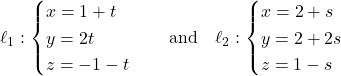
- 2.

- 3.

For each problem below, apply the point-to-plane distance formula to calculate the shortest perpendicular distance from the given point  to the plane .
- 1. Point
 and plane
- 2. Point
 and plane
- 3. Point
 and plane
Verify that each pair of planes below is parallel, choose an arbitrary reference point on the first plane, and calculate the shortest distance separating them.
- 1.

- 2.

- 3.

For each pair of skew lines below, use either the orthogonality dot product system or the scalar triple product formula to determine the shortest geometric distance separating them in .
- 1.

- 2.
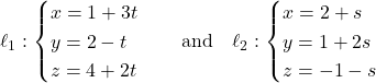
- 3.
