We know from using the Newton-Leibniz theorem that the area under the curve of a function  with primitive
  taken from
  to
to  is given by:
![\[\int_a^bf(x)dx=F(b)-F(a)\]](https://mathematics.lu/wp-content/ql-cache/quicklatex.com-300133fef82513d50118f489b9f9b379_l3.png "Rendered by QuickLaTeX.com")
The reality is that we need to adapt this depending on the function. This formula represents the net area between the curve of a function
and the  -axis.
Motivation
Say we want to find the total area enclosed between the graph of  and the -axis from
  to
to  .
.
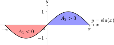
If we blindly compute the definite integral across the entire interval using the Newton-Leibniz formula, we get:
![\[\int_{-\pi}^{\pi} \sin(x) \, dx = \Big[ -\cos(x) \Big]_{-\pi}^{\pi} = \underbrace{-\cos(\pi)}_{1} - \underbrace{\big(-\cos(-\pi)\big)}_{1} = 1 - 1 = 0\]](https://mathematics.lu/wp-content/ql-cache/quicklatex.com-b6900e7427d01318cb3d41f3b89a32b7_l3.png "Rendered by QuickLaTeX.com")
However, the total physical area cannot be zero because we see two regions and area is always non-negative.
How do we fix this? The problem comes from our function changing sign within the given interval. Therefore, if we put our function in absolute value, that will fix our problem. However, this is only helpful when we have a calculator to find the integral. We should still learn how to do this without relying on a calculator.
Total Area
To fix our opening problem, we follow the steps below:
- Separate the integral into appropriate intervals: Identify where the function changes signs by finding its roots (-intercepts).
- Set up the area formula with a minus sign for negative regions: To prevent cancellation, we place a minus sign in front of every integral for which the function is below the -axis in that interval of integration.
- Evaluate each integral separately via Newton-Leibniz.
- Add the results.
Example: Find the total area enclosed between the graph of and the -axis from to .
The definite integral tracks signed area. On the interval ![[-\pi, 0]](https://mathematics.lu/wp-content/ql-cache/quicklatex.com-962a1861f57c66f6e91ed5e8e8e8dd1d_l3.png "Rendered by QuickLaTeX.com") , the function dips below the -axis, yielding a negative integral value (
, the function dips below the -axis, yielding a negative integral value ( ). On
). On ![[0, \pi]](https://mathematics.lu/wp-content/ql-cache/quicklatex.com-96c8ad6f78ead72528c6b4bf3752193a_l3.png "Rendered by QuickLaTeX.com") , the function stays above the axis, yielding an equal positive value (
, the function stays above the axis, yielding an equal positive value ( ). When integrated as a single piece, these regions cancel each other out (
 ).
).
 at
at ![\[\text{Total Area} = -\int_{-\pi}^{0} \sin(x) \, dx + \int_{0}^{\pi} \sin(x) \, dx\]](https://mathematics.lu/wp-content/ql-cache/quicklatex.com-4798ae97f9c263f180240ad8a40c8d90_l3.png "Rendered by QuickLaTeX.com")
![\[\text{Total Area} = -\Big[ -\cos(x) \Big]_{-\pi}^{0} + \Big[ -\cos(x) \Big]_{0}^{\pi}\]](https://mathematics.lu/wp-content/ql-cache/quicklatex.com-37902a52afbdc3b6f78d4d8b167ce51f_l3.png "Rendered by QuickLaTeX.com")
![\[\text{Total Area} = -\Big( -\cos(0) - (-\cos(-\pi)) \Big) + \Big( -\cos(\pi) - (-\cos(0)) \Big)\]](https://mathematics.lu/wp-content/ql-cache/quicklatex.com-eb1b44c23738b4e4bb0061591be30baa_l3.png "Rendered by QuickLaTeX.com")
![\[\text{Total Area} = -\Big( -1 - 1 \Big) + \Big( -(-1) - (-1) \Big)\]](https://mathematics.lu/wp-content/ql-cache/quicklatex.com-3501bc4dc75d156060df386f685a029d_l3.png "Rendered by QuickLaTeX.com")
![\[\text{Total Area} = -(-2) + 2 = 2 + 2 = 4\]](https://mathematics.lu/wp-content/ql-cache/quicklatex.com-719d4fee62cead0309b403552f8fd642_l3.png "Rendered by QuickLaTeX.com")
Example: Below is the graph of  . Find the total geometric area enclosed between and the -axis from
  to
to  .
.
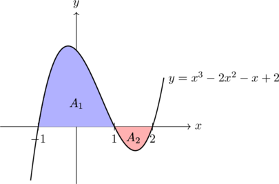
 reveals the roots at
 ![[-1, 1]](https://mathematics.lu/wp-content/ql-cache/quicklatex.com-66c17e240f5e7fd4ea51af9e1301d35e_l3.png "Rendered by QuickLaTeX.com") and dips below the
and dips below the ![[1, 2]](https://mathematics.lu/wp-content/ql-cache/quicklatex.com-6a1f4ecd197bf9d62f6c007c1d518b5e_l3.png "Rendered by QuickLaTeX.com") . We must split our area computation into these two sub-intervals.
. We must split our area computation into these two sub-intervals.![\[\text{Total Area} = \int_{-1}^{1} (x^3 - 2x^2 - x + 2) \, dx - \int_{1}^{2} (x^3 - 2x^2 - x + 2) \, dx\]](https://mathematics.lu/wp-content/ql-cache/quicklatex.com-dd9789fdc6e397e1813996ece886947d_l3.png "Rendered by QuickLaTeX.com")
![\[F(x) = \frac{x^4}{4} - \frac{2x^3}{3} - \frac{x^2}{2} + 2x\]](https://mathematics.lu/wp-content/ql-cache/quicklatex.com-0ad8b2adce5a02df4816099e3839066d_l3.png "Rendered by QuickLaTeX.com")
![\[F(1) = \frac{1}{4} - \frac{2}{3} - \frac{1}{2} + 2 = \frac{3 - 8 - 6 + 24}{12} = \frac{13}{12}\]](https://mathematics.lu/wp-content/ql-cache/quicklatex.com-35bdc2ceddb1ee3621c22bf82ca2c27d_l3.png "Rendered by QuickLaTeX.com")
![\[F(-1) = \frac{1}{4} + \frac{2}{3} - \frac{1}{2} - 2 = \frac{3 + 8 - 6 - 24}{12} = -\frac{19}{12}\]](https://mathematics.lu/wp-content/ql-cache/quicklatex.com-b7cbf827d7cf81c8028f95f5c2c5cb8d_l3.png "Rendered by QuickLaTeX.com")
![\[F(2) = \frac{16}{4} - \frac{16}{3} - \frac{4}{2} + 4 = 4 - \frac{16}{3} - 2 + 4 = 6 - \frac{16}{3} = \frac{2}{3} = \frac{8}{12}\]](https://mathematics.lu/wp-content/ql-cache/quicklatex.com-684875be583a3ab7484aae364f278e83_l3.png "Rendered by QuickLaTeX.com")
![\[A_1 = F(1) - F(-1) = \frac{13}{12} - \left(-\frac{19}{12}\right) = \frac{32}{12} = \frac{8}{3}\]](https://mathematics.lu/wp-content/ql-cache/quicklatex.com-d102913b3e56cb38dff4270062e04320_l3.png "Rendered by QuickLaTeX.com")
![\[A_2 = F(2) - F(1) = \frac{8}{12} - \frac{13}{12} = -\frac{5}{12}\]](https://mathematics.lu/wp-content/ql-cache/quicklatex.com-0bf10b7bc4fa9cf6d721a617ca544e49_l3.png "Rendered by QuickLaTeX.com")
![\[\text{Total Area} = A_1 - A_2 = \frac{32}{12} - \left(-\frac{5}{12}\right) = \frac{37}{12} \approx 3.083\]](https://mathematics.lu/wp-content/ql-cache/quicklatex.com-114fd3aaca026efb39f7f17ebf37aff9_l3.png "Rendered by QuickLaTeX.com")
We can either find  and
and  as areas (and so they cannot be negative) and simply say
![\[Area=A_1+A_2\]](https://mathematics.lu/wp-content/ql-cache/quicklatex.com-6339267be4b3b07809acff89bf3d8403_l3.png "Rendered by QuickLaTeX.com")
Or find
and as integrals (so will be negative because the function is below the -axis) and then subtract them, as in the example above.We may not always be given the graph of the function, so it may be up to use to understand if it is above the
-axis or below the -axis in each interval.
Area Between Curves
If we are given two functions and  and asked for the area between them, it is implied that these functions will intersect. To find the area between the two functions, we could find the area below the graph of a function, the area below the other, and subtract them. However, an easier approach would be to take the difference of functions. This will be a new function and the area between this new function and the -axis is equivalent to the area between the functions.
The only problem with this is that we need to account for where the new function is positive/negative. This is the same as understand which function  or
or  is the greater one.
Example: Find the total geometric area enclosed between the cubic polynomial  and the linear function
  .
.
To see where the curves cross and which function sits on top over different intervals, let us inspect the graph below:
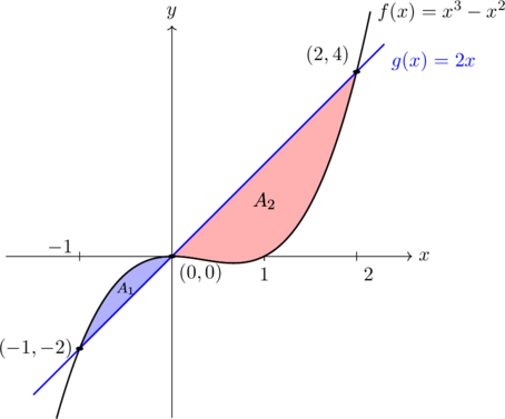
![\[x^3 - x^2 = 2x \implies x^3 - x^2 - 2x = 0\]](https://mathematics.lu/wp-content/ql-cache/quicklatex.com-bd160d320e061ea6288658e96da030a0_l3.png "Rendered by QuickLaTeX.com")
![\[x(x^2 - x - 2) = 0 \implies x(x - 2)(x + 1) = 0\]](https://mathematics.lu/wp-content/ql-cache/quicklatex.com-bd596bd6d76b4459ec2292dfaad2f1d9_l3.png "Rendered by QuickLaTeX.com")
![[-1, 0]](https://mathematics.lu/wp-content/ql-cache/quicklatex.com-084e50e9dcc4282931315aa2a6337d2e_l3.png "Rendered by QuickLaTeX.com") and
and ![[0, 2]](https://mathematics.lu/wp-content/ql-cache/quicklatex.com-e250a581660e7bfe3221162fa4497625_l3.png "Rendered by QuickLaTeX.com") .
.![\[\text{Total Area} = A_1 + A_2 = \int_{-1}^{0} \big( (x^3 - x^2) - 2x \big) \, dx + \int_{0}^{2} \big( 2x - (x^3 - x^2) \big) \, dx\]](https://mathematics.lu/wp-content/ql-cache/quicklatex.com-334540d854c2c2f35d3432134d2c619c_l3.png "Rendered by QuickLaTeX.com")
![\[\text{Total Area} = \int_{-1}^{0} (x^3 - x^2 - 2x) \, dx + \int_{0}^{2} (-x^3 + x^2 + 2x) \, dx\]](https://mathematics.lu/wp-content/ql-cache/quicklatex.com-ca0738bdadfb68578fb6352163631cee_l3.png "Rendered by QuickLaTeX.com")
![\[\text{First Primitive } F_1(x) = \frac{x^4}{4} - \frac{x^3}{3} - x^2\]](https://mathematics.lu/wp-content/ql-cache/quicklatex.com-160c6b1906c39d70a5ba2f24fd4d4f9b_l3.png "Rendered by QuickLaTeX.com")
![\[\text{Second Primitive } F_2(x) = -\frac{x^4}{4} + \frac{x^3}{3} + x^2\]](https://mathematics.lu/wp-content/ql-cache/quicklatex.com-be5e5b23baf9657ef161a729cccaf6a9_l3.png "Rendered by QuickLaTeX.com")
![\[F_1(0) = 0\]](https://mathematics.lu/wp-content/ql-cache/quicklatex.com-5e4c51c6bb41d4a90496ae29d36f265b_l3.png "Rendered by QuickLaTeX.com")
![\[F_1(-1) = \frac{(-1)^4}{4} - \frac{(-1)^3}{3} - (-1)^2 = \frac{1}{4} + \frac{1}{3} - 1 = \frac{3 + 4 - 12}{12} = -\frac{5}{12}\]](https://mathematics.lu/wp-content/ql-cache/quicklatex.com-e81d9757f9b25596c0e9ffd35daaa359_l3.png "Rendered by QuickLaTeX.com")
![\[A_1 = F_1(0) - F_1(-1) = 0 - \left(-\frac{5}{12}\right) = \frac{5}{12}\]](https://mathematics.lu/wp-content/ql-cache/quicklatex.com-6ded46883e8515ed48b2fbd3f06717ef_l3.png "Rendered by QuickLaTeX.com")
![\[F_2(2) = -\frac{2^4}{4} + \frac{2^3}{3} + 2^2 = -4 + \frac{8}{3} + 4 = \frac{8}{3} = \frac{32}{12}\]](https://mathematics.lu/wp-content/ql-cache/quicklatex.com-da6feda3957f2f008f5ad82a5297a7ef_l3.png "Rendered by QuickLaTeX.com")
![\[F_2(0) = 0\]](https://mathematics.lu/wp-content/ql-cache/quicklatex.com-df8c56098fe7212624ab851a13c60eb7_l3.png "Rendered by QuickLaTeX.com")
![\[A_2 = F_2(2) - F_2(0) = \frac{32}{12} - 0 = \frac{32}{12}\]](https://mathematics.lu/wp-content/ql-cache/quicklatex.com-a1c83dd9881d8568395ec0c079a5a820_l3.png "Rendered by QuickLaTeX.com")
![\[\text{Total Area} = \frac{5}{12} + \frac{32}{12} = \frac{37}{12} \approx 3.083\]](https://mathematics.lu/wp-content/ql-cache/quicklatex.com-63f9468225bf93aeb64a53093718eb75_l3.png "Rendered by QuickLaTeX.com")
Solid of Revolution
This formula is used to calculate the three-dimensional space (volume) inside a solid object that has a perfectly circular cross-section, like a vase, a funnel, a bowl, or a cone. In calculus, these shapes are called solids of revolution. Imagine you have a flat, 2D shape drawn on a piece of paper. The top boundary of this shape is your curve , the bottom boundary is the straight line of the -axis, and the sides are blocked off from to .
Now, imagine sticking a straight metal skewer directly along the -axis and spinning the paper at a full 360-degree rotation. As that flat 2D shape sweeps through the air while spinning, it carves out a solid, 3D object in space. The straight line along the -axis stays completely still, forming the solid core centre of the object.
The curve spins through the air, forming the smooth outer crust/shell of the object.
Theorem (Volume of a Solid of Revolution – Disk Method): Let be a continuous and non-negative function on the closed interval ![[a, b]](https://mathematics.lu/wp-content/ql-cache/quicklatex.com-458a76d7f1dc15e9dc8be46976f8197d_l3.png "Rendered by QuickLaTeX.com") . When the region enclosed under the curve
. When the region enclosed under the curve  and the -axis is rotated
  around the -axis, the volume
  of the resulting three-dimensional solid is given by:
![\[V = \pi \int_a^b \big[f(x)\big]^2 \, dx\]](https://mathematics.lu/wp-content/ql-cache/quicklatex.com-6cfd2a1fbc9d966d7592e399a2a92084_l3.png "Rendered by QuickLaTeX.com")
For background: This formula treats the solid as a collection of infinitely thin cylindrical disks with radius  and thickness
  , where the area of each circular cross-section is
 ![\pi r^2 = \pi \big[f(x)\big]^2](https://mathematics.lu/wp-content/ql-cache/quicklatex.com-112cb8848646edc9e2fd92f9f7382793_l3.png "Rendered by QuickLaTeX.com") . Let us see this used in an example.
. Let us see this used in an example.
Example: Find the volume of the solid generated by revolving the region bounded by the curve  , the -axis,
  , and
, and  around the -axis.
 is spun
 ![V = \pi \int_a^b [f(x)]^2 dx](https://mathematics.lu/wp-content/ql-cache/quicklatex.com-40b4553c7fa8f34a1062166498fb56fa_l3.png "Rendered by QuickLaTeX.com") . Plugging in our boundaries (
. Plugging in our boundaries ( ,
,  ) and our radius function
  gives:
![\[V = \pi \int_1^4 \big(x^2\big)^2 \, dx\]](https://mathematics.lu/wp-content/ql-cache/quicklatex.com-9d10671f94ddf23688c38a7236bf05dc_l3.png "Rendered by QuickLaTeX.com")
 ) simplifies the expression inside the integral:
![\[V = \pi \int_1^4 x^4 \, dx\]](https://mathematics.lu/wp-content/ql-cache/quicklatex.com-64079b43d9c41392fb81a6d35b2a0e21_l3.png "Rendered by QuickLaTeX.com")
 gives
gives  :
:![\[V = \pi \left[ \frac{x^5}{5} \right]_1^4\]](https://mathematics.lu/wp-content/ql-cache/quicklatex.com-d44bc56317092eb5d0bf582392a0d75a_l3.png "Rendered by QuickLaTeX.com")
 and subtract the lower bound at
  :
:![\[V = \pi \left( \frac{4^5}{5} - \frac{1^5}{5} \right)\]](https://mathematics.lu/wp-content/ql-cache/quicklatex.com-38b1a3736f1e6aec3ff2668b9dda119b_l3.png "Rendered by QuickLaTeX.com")
![\[V = \pi \left( \frac{1024}{5} - \frac{1}{5} \right)\]](https://mathematics.lu/wp-content/ql-cache/quicklatex.com-7c7f208ddf8ef692b6c993c8b1ca85dd_l3.png "Rendered by QuickLaTeX.com")
![\[V = \pi \left( \frac{1023}{5} \right) = 204.6\pi \approx 642.77 \text{ cubic units}\]](https://mathematics.lu/wp-content/ql-cache/quicklatex.com-cb67160327dbadccfef5681e69d23a62_l3.png "Rendered by QuickLaTeX.com")
Famous Volume Formula
In this section, we will use our knowledge of integrals and volumes to prove the formula for the volume of a sphere (as seen in S5).
Example: Prove the classical geometric formula for the volume of a sphere using the calculus disk method by revolving the upper semicircle  from to around the -axis.
To help visualize how a 2D boundary curve spins to construct a perfect 3D sphere, let us look at the upper semicircle function graph below:
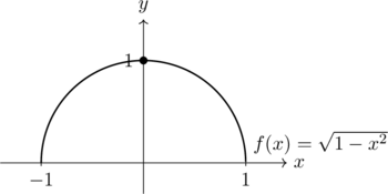
 is rotated
  ,
,  ) and our upper boundary height radius function
 ![\[V = \pi \int_{-1}^{1} \left(\sqrt{1 - x^2}\right)^2 \, dx\]](https://mathematics.lu/wp-content/ql-cache/quicklatex.com-86544f06126ff66842b73be8f465f8a3_l3.png "Rendered by QuickLaTeX.com")
![\[V = \pi \int_{-1}^{1} (1 - x^2) \, dx\]](https://mathematics.lu/wp-content/ql-cache/quicklatex.com-63e2968d9004cc62f7092a27b3c78fba_l3.png "Rendered by QuickLaTeX.com")
![\[V = \pi \left[ x - \frac{x^3}{3} \right]_{-1}^{1}\]](https://mathematics.lu/wp-content/ql-cache/quicklatex.com-de9fb2fbd3fa8b141a998744626caaa5_l3.png "Rendered by QuickLaTeX.com")
![\[V = \pi \left( \left(1 - \frac{1^3}{3}\right) - \left(-1 - \frac{(-1)^3}{3}\right) \right)\]](https://mathematics.lu/wp-content/ql-cache/quicklatex.com-25316f9261f703ff854d96ebde45440c_l3.png "Rendered by QuickLaTeX.com")
![\[V = \pi \left( \left(1 - \frac{1}{3}\right) - \left(-1 + \frac{1}{3}\right) \right)\]](https://mathematics.lu/wp-content/ql-cache/quicklatex.com-8225aaa344dbc04c8d74ea632b42b72b_l3.png "Rendered by QuickLaTeX.com")
![\[V = \pi \left( \frac{2}{3} - \left(-\frac{2}{3}\right) \right) = \pi \left( \frac{2}{3} + \frac{2}{3} \right) = \frac{4}{3}\pi \text{ cubic units}\]](https://mathematics.lu/wp-content/ql-cache/quicklatex.com-fd9734a1ce804cd28f8c12f9fe884731_l3.png "Rendered by QuickLaTeX.com")
 into our starting algebraic boundary equation (
 from
from  to
to ![\[V = \frac{4}{3}\pi R^3\]](https://mathematics.lu/wp-content/ql-cache/quicklatex.com-9af514b61ca6a85006e8f5e986fa0e4b_l3.png "Rendered by QuickLaTeX.com")
Gabriel’s Horn/Torricelli’s Trumpet
We finish our exploration into volume calculation with a famous example. Torricelli’s Trumpet is a famous mathematical paradox. It describes an infinitely long geometric solid that has a finite volume but an infinite surface area.
Evaluate the volume and surface area of Torricelli’s Trumpet (Gabriel’s Horn), generated by rotating the curve  from to
  around the -axis.
2D Cross-Section Profile
3D Solid Revolution
Part 1: Volume Calculation
The general formula for the volume of a solid of revolution is ![V = \pi \int_a^b [f(x)]^2 \, dx](https://mathematics.lu/wp-content/ql-cache/quicklatex.com-59cb527d02616d3a26debaabc83558ce_l3.png "Rendered by QuickLaTeX.com") . Setting the boundaries from
. Setting the boundaries from  to
to  yields:
![\[V = \pi \int_1^\infty \left(\frac{1}{x}\right)^2 \, dx = \pi \lim_{b \to \infty} \int_1^b x^{-2} \, dx\]](https://mathematics.lu/wp-content/ql-cache/quicklatex.com-b8f0c8277954994891ceac3003a0ed44_l3.png "Rendered by QuickLaTeX.com")
Applying the power rule for integration:
![\[V = \pi \lim_{b \to \infty} \left[ -\frac{1}{x} \right]_1^b = \pi \lim_{b \to \infty} \left( -\frac{1}{b} - \left(-\frac{1}{1}\right) \right)\]](https://mathematics.lu/wp-content/ql-cache/quicklatex.com-ab522bcfddac968662fffde65e9b5f12_l3.png "Rendered by QuickLaTeX.com")
Evaluating the limit as  reveals a finite volume:
![\[V = \pi (0 + 1) = \pi \text{ cubic units}\]](https://mathematics.lu/wp-content/ql-cache/quicklatex.com-8a808e76366522c920ddcf40e0fc3b82_l3.png "Rendered by QuickLaTeX.com")
Part 2: Surface Area Calculation
The general formula for the surface area (not in the programme) of a solid of revolution around the -axis is:
![\[S = 2\pi \int_a^b f(x) \sqrt{1 + \big[f'(x)\big]^2} \, dx\]](https://mathematics.lu/wp-content/ql-cache/quicklatex.com-7bf30c137d168c7ea186aa713613e5ce_l3.png "Rendered by QuickLaTeX.com")
For , the derivative is  . Setting up the surface area integral gives:
![\[S = 2\pi \int_1^\infty \frac{1}{x} \sqrt{1 + \left(-\frac{1}{x^2}\right)^2} \, dx = 2\pi \int_1^\infty \frac{1}{x} \sqrt{1 + \frac{1}{x^4}} \, dx\]](https://mathematics.lu/wp-content/ql-cache/quicklatex.com-0b02764352202b8ae2103503e91ae83c_l3.png "Rendered by QuickLaTeX.com")
Because the square root term  is strictly greater than for all
  , we can establish a lower-bound inequality:
![\[S > 2\pi \int_1^\infty \frac{1}{x} \, dx\]](https://mathematics.lu/wp-content/ql-cache/quicklatex.com-d371c24dd8182744ac0774fd04b761f0_l3.png "Rendered by QuickLaTeX.com")
Evaluating this integral over the infinite interval via natural logarithms:
![\[\int_1^\infty \frac{1}{x} \, dx = \lim_{b \to \infty} \int_1^b \frac{1}{x} \, dx = \lim_{b \to \infty} \Big[ \ln|x| \Big]_1^b = \lim_{b \to \infty} \big( \ln(b) - \ln(1) \big) = \infty - 0 = \infty\]](https://mathematics.lu/wp-content/ql-cache/quicklatex.com-aa57a0e2b384340bfb8ffd634dd4d64f_l3.png "Rendered by QuickLaTeX.com")
Since the lower bound diverges to infinity, the total surface area  is infinite:
![\[S = \infty \text{ square units}\]](https://mathematics.lu/wp-content/ql-cache/quicklatex.com-823e7222851a523f5ea1f589acbdc839_l3.png "Rendered by QuickLaTeX.com")
This implies you could fill the entire horn with a finite amount of paint, but that same amount of paint would not be enough to coat its outer surface!
Exercises
Find the exact geometric area enclosed between the graph of each function and the -axis over the given interval. Use the provided vector plots for reference.
1.  from
from  to
to  .
.
2.  from to .
3.  from to .
4.  from to
  .
.
5.  from to .
Find the area enclosed between the curves of the given functions. Determine their intersection points algebraically to find the limits of integration.
1. Enclosed by  and
and  .
.
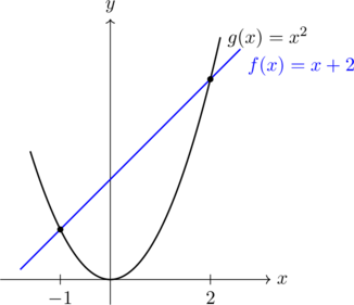
2. Enclosed by  and .
and .
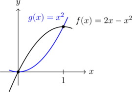
3. Enclosed by  and
and  .
.
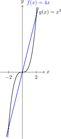
4. Enclosed by  and
and  .
.
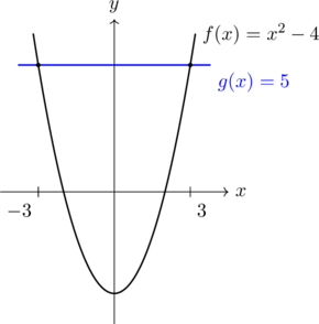
Calculate the volume of the solid generated by rotating the region bounded by the given curves around the -axis over the specified intervals.
1.  , the -axis, from to .
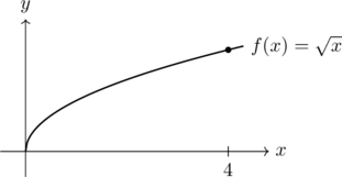
2. , the -axis, from to .
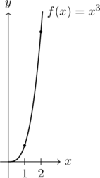
3. , the -axis, from to  .
.
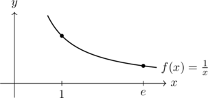
4. , the -axis, from to .
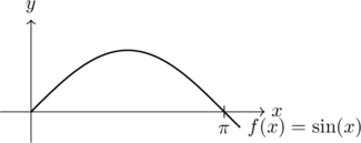
Prove the classical geometric volume formula for a cone,  , using the disk integration method.
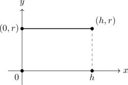
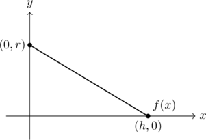
Consider a straight line starting at the point  on the
  -axis and slanting down to hit the -axis at the point
  . When the area beneath this linear profile line is spun around the -axis, it carves out a perfect cone with base radius
  and height
  . Refer to the graph below:
Steps to Complete the Proof:
- Find the equation of the line as a function of and .
- Use the formula for the solid of revolution volume with boundaries:
 and
and  .
. - Apply the Newton-Leibniz formula.
Prove the classical geometric volume formula for a cylinder,  , by applying the volume formula to the constant function
  from
from  to
to  .
.