Relative Position of Lines in 3D

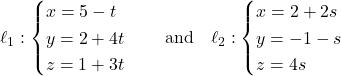
In this page, we discuss how different lines can interact.

Table of Contents

Parallel Lines

Definition (Parallel Lines in $\mathbb{R}^3$ ): Two lines in a three-dimensional space are parallel if and only if their corresponding direction vectors are parallel, i.e.: one direction vector is a scalar multiple of the other.

$\ell_1 \parallel \ell_2 \iff \vec{d}_1 = k\vec{d}_2 \quad (k \neq 0)$

With $v_1$ and $v_2$ being the direction vectors of $\ell_1$ and $\ell_2$ .

Example: Show that the two lines $\ell_1$ and $\ell_2$ are parallel lines:

$\ell_1: \begin{cases} x = 2 + t \\ y = -1 + 3t \\ z = 4 - 2t \end{cases} \quad \text{and} \quad \ell_2: \frac{x - 5}{-2} = \frac{y - 1}{-6} = \frac{z + 3}{4}$

Example: Determine whether the two lines $\ell_1$ and $\ell_2$ are parallel lines:

$\ell_1: \begin{cases} x = 1 + 2t \\ y = -3 - 4t \\ z = 5 + 6t \end{cases} \quad \text{and} \quad \ell_2: \frac{x - 3}{-1} = \frac{y - 2}{2} = \frac{z + 4}{-3}$

In particular, two lines are called coinciding/coincident if they are parallel and they share a point. If two parallel lines share a point, then they must share infinite points, and therefore be the same line. That is what this last definition says.

Example: Determine whether the two lines $\ell_1$ and $\ell_2$ are coinciding lines:

$\ell_1: \begin{pmatrix} x \\ y \\ z \end{pmatrix} = \begin{pmatrix} 1 \\ 2 \\ -1 \end{pmatrix} + t\begin{pmatrix} 3 \\ -1 \\ 2 \end{pmatrix} \quad \text{and} \quad \ell_2: \frac{x - 4}{6} = \frac{y - 1}{-2} = \frac{z - 1}{4}$

Intersecting Lines

Two lines are called intersecting if they share a point. To find the intersection between two lines, we create a system of equations that will make their $x,y,$ and $z$ coordinates equal. This will result in a system with 2 variables (the parameters of each line) and 3 equations. As we know, this could yield either: no solution, 1 exact solution, infinite solutions. Each of these yields a relative position between lines.

The calculator can help us solve this system, but we can also tackle it without a technological tool. To do so, solve the system by using the first two equations (ignore the third one). This should yield a value for your variables, check that the third equation is consistent with that value. If it is, the lines intersect. Otherwise, they lines do not.

Example: Prove that the two lines $\ell_1$ and $\ell_2$ intersect, and determine their single point of intersection:

$\ell_1: \begin{cases} x = 1 + t \\ y = -2 + 2t \\ z = 4 - t \end{cases} \quad \text{and} \quad \ell_2: \begin{cases} x = 2 + s \\ y = -1 + 3s \\ z = 1 + s \end{cases}$

Example: Determine whether the two lines $\ell_1$ and $\ell_2$ intersect, are parallel, or are skew:

$\ell_1: \begin{cases} x = 1 + t \\ y = -2 + 2t \\ z = 4 - t \end{cases} \quad \text{and} \quad \ell_2: \begin{cases} x = 2 + s \\ y = 3 + 4s \\ z = 1 + s \end{cases}$

Skew Lines

This position did not exist in 3 dimensions. Two lines that are not parallel and do not intersect are called skew lines. Our default way to show that two lines are skew is to show that they are not parallel (by comparing their direction vectors) and that they do not intersect (by getting a system of equations with no solution).

Rendered by QuickLaTeX.com

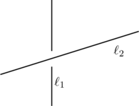
The example above showed two skew lines, but we can see another one.

Example: Show that the two lines $\ell_1$ and $\ell_2$ are skew lines:

$\ell_1: \begin{cases} x = 2 + 3t \\ y = 1 - t \\ z = 5 + 2t \end{cases} \quad \text{and} \quad \ell_2: \begin{cases} x = -1 + t \\ y = 4 + 2t \\ z = 3 - t \end{cases}$

Notice that skew lines are not parallel. In the past, you have probably defined parallel lines as lines that never intersect. That is a nice intuitive definition but, as you can see in 3 dimensions, this is no longer applicable. It is true, in 2 dimensions, that lines either intersect or are parallel, but in $\mathbb{R}^3$ we have this third option.

Angle Between Two Lines

We already discussed the formula for the acute angle $\theta$ created by two vectors $\vec{u}$ and $\vec{v}$ . This is:

$\cos(\theta)=\frac{\vec{u}\cdot\vec{v}}{\|\vec{u}\|\cdot\|\vec{v}\|}\implies\theta=\arccos\left(\frac{\vec{u}\cdot\vec{v}}{\|\vec{u}\|\cdot\|\vec{v}\|}\right)$

Definition (Angle Between Two Lines): The angle $\theta$ between two intersecting or skew lines $\ell_1$ and $\ell_2$ is defined as the acute angle formed by their respective direction vectors $\vec{d}_1$ and $\vec{d}_2$ .

$\cos(\theta) = \frac{|\vec{d}_1 \cdot \vec{d}_2|}{\|\vec{d}_1\| \|\vec{d}_2\|} \quad \text{where} \quad \theta \in \left[0, \frac{\pi}{2}\right]$

Example: Calculate the acute angle $\theta$ between the two lines $\ell_1$ and $\ell_2$ :

$\ell_1: \begin{cases} x = 1 + 2t \\ y = -t \\ z = 3 + 2t \end{cases} \quad \text{and} \quad \ell_2: \frac{x - 4}{1} = \frac{y + 2}{2} = \frac{z - 1}{2}$

Exercises

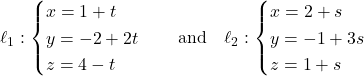
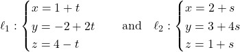
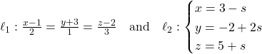
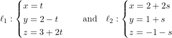
For each pair of lines below, analyze their direction vectors and coordinate systems to classify their relative spatial position as parallel, coincident, intersecting, or skew. If the lines intersect, determine their specific point of intersection.

1. $\ell_1: \begin{cases} x = 1 + t \\ y = -2 + 2t \\ z = 4 - t \end{cases} \quad \text{and} \quad \ell_2: \begin{cases} x = 2 + s \\ y = -1 + 3s \\ z = 1 + s \end{cases}$
2. $\ell_1: \begin{cases} x = 2 + t \\ y = -1 + 3t \\ z = 4 - 2t \end{cases} \quad \text{and} \quad \ell_2: \frac{x - 5}{-2} = \frac{y - 1}{-6} = \frac{z + 3}{4}$
3. $\ell_1: \begin{pmatrix} x \\ y \\ z \end{pmatrix} = \begin{pmatrix} 1 \\ 2 \\ -1 \end{pmatrix} + t\begin{pmatrix} 3 \\ -1 \\ 2 \end{pmatrix} \quad \text{and} \quad \ell_2: \frac{x - 4}{6} = \frac{y - 1}{-2} = \frac{z - 1}{4}$
4. $\ell_1: \begin{cases} x = 1 + t \\ y = -2 + 2t \\ z = 4 - t \end{cases} \quad \text{and} \quad \ell_2: \begin{cases} x = 2 + s \\ y = 3 + 4s \\ z = 1 + s \end{cases}$
5. $\ell_1: \frac{x - 1}{2} = \frac{y + 3}{1} = \frac{z - 2}{3} \quad \text{and} \quad \ell_2: \begin{cases} x = 3 - s \\ y = -2 + 2s \\ z = 5 + s \end{cases}$
6. $\ell_1: \begin{pmatrix} x \\ y \\ z \end{pmatrix} = \begin{pmatrix} 0 \\ 4 \\ 1 \end{pmatrix} + t\begin{pmatrix} 1 \\ -1 \\ 2 \end{pmatrix} \quad \text{and} \quad \ell_2: \frac{x - 2}{-2} = \frac{y - 2}{2} = \frac{z - 5}{-4}$
7. $\ell_1: \frac{x + 1}{3} = \frac{y - 2}{-1} = \frac{z - 4}{2} \quad \text{and} \quad \ell_2: \begin{pmatrix} x \\ y \\ z \end{pmatrix} = \begin{pmatrix} -4 \\ 3 \\ 2 \end{pmatrix} + s\begin{pmatrix} -3 \\ 1 \\ -2 \end{pmatrix}$
8. $\ell_1: \begin{cases} x = t \\ y = 2 - t \\ z = 3 + 2t \end{cases} \quad \text{and} \quad \ell_2: \begin{cases} x = 2 + 2s \\ y = 1 + s \\ z = -1 - s \end{cases}$
9. $\ell_1: \frac{x - 2}{4} = \frac{y + 1}{-2} = \frac{z - 3}{6} \quad \text{and} \quad \ell_2: \frac{x - 4}{-2} = \frac{y + 2}{1} = \frac{z - 6}{-3}$
10. $\ell_1: \begin{pmatrix} x \\ y \\ z \end{pmatrix} = \begin{pmatrix} 1 \\ 0 \\ 2 \end{pmatrix} + t\begin{pmatrix} 2 \\ 1 \\ -1 \end{pmatrix} \quad \text{and} \quad \ell_2: \begin{cases} x = 2 + s \\ y = -1 + s \\ z = 3 + 2s \end{cases}$

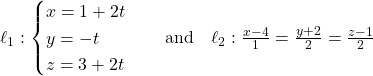
Extract the direction vectors for each pair of lines below and apply the acute angle formula to determine the exact angle $\theta$ between them.

1. $\ell_1: \begin{cases} x = 1 + 2t \\ y = -t \\ z = 3 + 2t \end{cases} \quad \text{and} \quad \ell_2: \frac{x - 4}{1} = \frac{y + 2}{2} = \frac{z - 1}{2}$
2. $\ell_1: \frac{x - 2}{3} = \frac{y + 1}{-4} = \frac{z}{0} \quad \text{and} \quad \ell_2: \begin{pmatrix} x \\ y \\ z \end{pmatrix} = \begin{pmatrix} 5 \\ 1 \\ -2 \end{pmatrix} + s\begin{pmatrix} 4 \\ 3 \\ -5 \end{pmatrix}$
3. $\ell_1: \begin{cases} x = 5 - t \\ y = 2 + 4t \\ z = 1 + 3t \end{cases} \quad \text{and} \quad \ell_2: \begin{cases} x = 2 + 2s \\ y = -1 - s \\ z = 4s \end{cases}$