In the previous page, we discussed an introduction to bivariate statistics. In essence, we are given two variables and asked what is the relation between them.
We have a way of finding the Pearson Correlation Coefficient, which describes more objectively whether the variables are positively/negatively correlated, and if the correlation is linear, non-linear, strong, weak, moderate, or even if there is no correlation at all between the variables.
Moreover, we have as a goal to generalise the behaviour/trend of the data to predict other values.
Least Squares Regression Line
Just like the Pearson Correlation Coefficient gives an objective way to describe the correlation, the least squares regression line gives an objective line of best fit.
Say we have our scatter plot and some line of best fit. The least squares regression line will be defined as that which minimises the squares of the vertical distance between each point and the regression line.
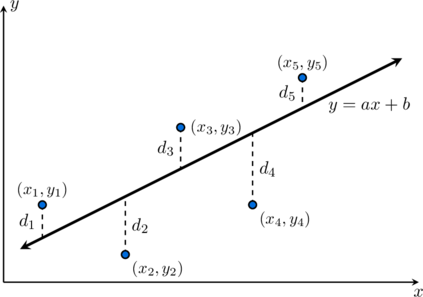
Though you can prove what the formulas for  and
 in this line are, this is not necessary. Your calculator will be able to give you a line of best fit following this model and we can use this line to interpolate/extrapolate.
Example: A local library monitors how the number of promotional community events hosted ( ) over several months relates to the total number of new membership registrations (
 , in hundreds). The collected bivariate data is displayed in the table below:
| Month | 1 | 2 | 3 | 4 | 5 | 6 |
|---|---|---|---|---|---|---|
| Events () |
2 | 4 | 5 | 7 | 8 | 10 |
| Registrations () |
15 | 22 | 21 | 31 | 30 | 39 |
- Draw a scatter plot for this dataset and sketch a line of best fit through the points.
- Find the equation of the least-squares regression line using a statistical calculator.
- Predict the membership registrations () if the library hosts
 events.
- Predict the number of events () required to secure
 hundred registrations.
- Comment on the reliability of your predictions in parts (c) and (d).
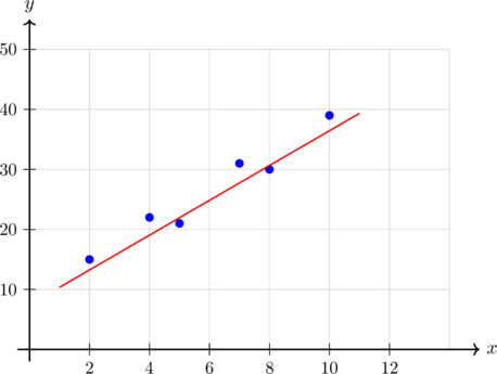



 hundred (
 memberships).



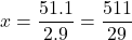
 community events.
 ). This is an example of interpolation. Conversely, the prediction in part (d) is much less reliable because
 (approximately
 ), which lies well outside the recorded field. This is an example of extrapolation, which assumes the current linear behaviour remains fixed indefinitely regardless of operational limits.
Regression line of a variable against another (Optional)
The only problem with the previous method for the least squares regression line is that there is an underlying assumption in doing so that the variable carries more accurate information, since looking at y variables and their distance from the line would technically include the error as well. For some instances, the -values may be more accurate.
When a student prepares for a test, if is the time spent studying and is the test score, we have that depends on . However, could obviously be measured more accurately than . Students could count the time they took a break, watched something, distracted themselves, answered a phone call, without knowing this when submitting the information. The score, however, is somewhat more objective.
In scenarios as above, we consider the regression line of against . This means that we minimise the squares of the horizontal distances of points from the line, so the error is associated with and not . The method is the same, we simply replace the roles of and in our scatter diagram.
Example: A manufacturing plant monitors the number of precision components produced () and the volume of chemical coolant consumed (, in litres) across 8 different production shifts. The data is recorded in the table below:
| Shift | 1 | 2 | 3 | 4 | 5 | 6 | 7 | 8 |
|---|---|---|---|---|---|---|---|---|
| Coolant (, litres) |
1.5 | 2.1 | 2.5 | 2.7 | 3.1 | 3.7 | 4.1 | 4.3 |
| Components () |
1 | 2 | 3 | 4 | 5 | 6 | 7 | 8 |
- Explain why it would be appropriate to use the regression line of against in this case.
- Find the regression line of against .
- Use the regression line to estimate the volume of coolant required to produce
 components.
- Use the regression line to estimate the number of components produced when
 of coolant are consumed.

 Components


 into the model and rearrange algebraically to isolate



This is basically the same principle of the least squares regression line but basing it on your more reliable variable. Just an alternative way to make predictions and find a model, albeit less used.
Other Regression Models
Your calculator might be able to show you different regression models and shapes that might fit your data more clearly. Imagine a Physics lab trying to prove, via an experiment, the acceleration of gravity. Throwing an object in the air, and measuring the height of the object as a function of time. We see that the height might increase as the time increases, but this trend will definitely not last forever. Therefore, a linear model is no longer suitable to represent the data. Instead, a quadratic model could be more appropriate.
Similarly, we could end up using an exponential model, or a logarithmic one.
Example: We are interested in studying the relationship between age and annual income (in thousands of euros). The table below presents data collected from a group of individuals:
Age ( , years) |
Yearly Income ( ) |
|---|---|
| 20 | 12 |
| 30 | 28 |
| 40 | 36 |
| 50 | 34 |
| 60 | 25 |
| 70 | 14 |
- Represent the data graphically on a scatter plot.
- Compute the linear regression line of income on age and discuss the quality of the fit.
- Compute the quadratic regression of on and compare its fit to the linear model.
- Using the quadratic interpretation, at what point would the maximum yearly income be achieved?
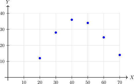

 , there is practically no linear correlation between age and annual income. A straight line is an exceptionally poor fit for this dataset, as confirmed by looking at the curved shape of the scatter plot.

 using the polynomial parameters:

Our final example will show a logarithmic regression. Just like this, there are many other regressions that may fit data more easily.
Example: A company tracks the relationship between the amount of money spent on online advertising (in thousands of euros) and the number of new customers acquired . The data collected are given below:
| Budget () |
New Customers () |
|---|---|
| 1 | 120 |
| 2 | 190 |
| 4 | 280 |
| 6 | 330 |
| 8 | 360 |
| 10 | 380 |
- Draw the scatter plot of the data.
- Discuss whether a linear model is appropriate.
Hint: does the increase in customers remain constant as the budget grows? - Fit a logarithmic regression model of the form
 .
- Use your model to predict the number of new customers when the advertising budget is
 thousand euros.
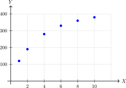
 , which indicates a strong positive linear link. However, examining the chart reveals diminishing returns: as the budget increases, the rate of customer acquisition decelerates rather than staying constant. Therefore, a purely linear model may misrepresent long-term system scaling parameters.

 , making it a significantly more accurate and appropriate description of the system trend line.



Exercises
An agricultural research team monitors the average daily greenhouse temperature (, in °C) and the weekly growth rate (, in mm) of a new test crop across six distinct thermal zones:
| Zone | 1 | 2 | 3 | 4 | 5 | 6 |
|---|---|---|---|---|---|---|
| Temperature () |
16 | 18 | 20 | 22 | 24 | 26 |
| Growth Rate () |
12 | 17 | 23 | 26 | 30 | 36 |
- 1. Draw a scatter plot for this dataset.
- 2. Calculate the correlation coefficient (
 ) using a calculator and describe the type of correlation.
- 3. Draw the line of best fit on your plot and find its equation using a calculator.
- 4. Predict the weekly growth rate () if the temperature is maintained at
 °C, and if it is raised to
 °C.
- 5. Comment on the reliability of your predictions in the previous step.
A tech startup tracks how the total number of software features added to a platform application () influences the engineering development time required (, in days) across six project modules:
| Module | A | B | C | D | E | F |
|---|---|---|---|---|---|---|
| Features () |
3 | 5 | 6 | 8 | 9 | 11 |
| Dev Time () |
14 | 22 | 23 | 31 | 32 | 40 |
- 1. Draw a scatter plot for this dataset.
- 2. Calculate the correlation coefficient () using a calculator and describe the type of correlation.
- 3. Draw the line of best fit on your plot and find its equation using a calculator.
- 4. Predict the total development days () needed to build a module containing
 features, and a module containing
 features.
- 5. Comment on the reliability of your predictions in the previous calculation.
A metallurgy lab tests how the continuous load runtime of a high-pressure valve system (, in hundreds of hours) impacts the micro-surface structural wear depth (, in microns) across six distinct components:
| Valve | 1 | 2 | 3 | 4 | 5 | 6 |
|---|---|---|---|---|---|---|
| Runtime () |
4 | 8 | 10 | 14 | 16 | 20 |
| Wear Depth () |
11 | 21 | 24 | 34 | 37 | 47 |
- 1. Draw a scatter plot for this dataset.
- 2. Calculate the correlation coefficient () using a calculator and describe the type of correlation.
- 3. Draw the line of best fit on your plot and find its equation using a calculator.
- 4. Predict the surface wear depth () at a runtime milestone of hundred hours, and if left running for
 hundred hours.
An agricultural research facility tracks how adding nitrogen-based fertiliser density (, in  ) impacts the net tomato harvest mass yield (, in kg) across six test plots:
| Plot | 1 | 2 | 3 | 4 | 5 | 6 |
|---|---|---|---|---|---|---|
| Fertiliser () |
10 | 20 | 30 | 40 | 50 | 60 |
| Yield () |
24 | 44 | 54 | 54 | 44 | 24 |
- 1. Draw a scatter plot for this dataset.
- 2. Calculate the correlation coefficient () using a calculator and describe the type of correlation.
- 3. Explain why a line of best fit is not appropriate here, and use a calculator to find the matching quadratic regression curve equation (
 ).
- 4. Predict the expected tomato harvest yield () for a fertiliser density inputs of
 , and an extreme density input of
 .
- 5. Comment on the reliability of your predictions.
A cognitive psychology experiment tracks the average word retention score (, out of 100) of a test cohort against the time elapsed since learning (, in hours) across six milestone windows:
| Window | 1 | 2 | 3 | 4 | 5 | 6 |
|---|---|---|---|---|---|---|
| Time elapsed (, hours) |
1 | 2 | 4 | 6 | 8 | 10 |
| Retention Score () |
92.0 | 78.137 | 64.274 | 56.163 | 50.411 | 45.952 |
- 1. Draw a scatter plot for this dataset.
- 2. Calculate the correlation coefficient () using a calculator and describe the type of correlation.
- 3. Explain why a standard straight line of best fit fails to capture this trend profile, and use a calculator to find the logarithmic curve equation (
 ).
- 4. Predict the expected word retention score () exactly
 after learning, and after an extended gap of
 .
- 5. Comment on the reliability of your predictions.