Bivariate statistics studies how to variables may or may not be connected. Here we study whether two variables behave in a linear form with relation to one another, or if another model may be appropriate, and how to use this “best model” to predict values not given in our experiment. Some of the questions that may interest us are:
- Does X cause Y?
- Are the variables X and Y related? How?
- Is there a way to measure how connected two variables are?
Motivation
Consider the following opening problem: the ambient daily temperature and the total revenue from ice cream sales are recorded at a beachside kiosk over twelve days.
| Day | A | B | C | D | E | F | G | H | I | J | K | L |
|---|---|---|---|---|---|---|---|---|---|---|---|---|
Temperature ( , °C) |
11 | 15 | 16 | 19 | 13 | 20 | 12 | 10 | 21 | 17 | 14 | 14 |
Revenue ( , EUR) |
22 | 31 | 25 | 42 | 24 | 48 | 16 | 12 | 55 | 36 | 20 | 26 |
Our two variables are temperature and revenue. This type of data is called bivariate data because it involves two variables. We expect the daily revenue to depend directly on the ambient temperature. Hence, we call temperature the independent variable (or explanatory variable) and ice cream revenue the dependent variable (or response variable).
We represent this data using a scatter plot.
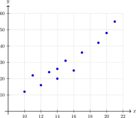
We can see that as temperature increases, the revenue increases. The question becomes in what form and what function best represents this data so that we could predict revenue/temperature based on the other variables.
Pearson’s Correlation Coefficient
The term correlation refers to the relationship or association between two numerical variables. There are several characteristics to consider when describing the correlation:
- Direction
- Strength
- Outliers
- Causation
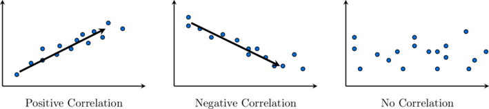
For a generally upward trend, we say that the correlation is positive. An increase in the independent variable (generally) results in an increase in the dependent variable. A generally downward trend shows a negative correlation. When the independent variable increases, the dependent variable decreases. If points are randomly scattered, we say there is no correlation. In short, we have:
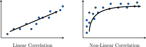
In terms of linearity, if a trend exists, we classify it either as linear or non-linear.
In terms of strength, we can have either strong, moderate, or weak (positive or negative) correlation. This is essentially a function of how close together your data is with relation to the line describing the correlation. Finally, we have causation. If a change in one variable causes a change in the other variable, we say that a causal relationship exists between them. Having correlation between two variables does not imply that one causes the other.
The Pearson Correlation Coefficient attempts to give a more objective way to determine how well data fits into a line.
Definition: Given a bivariate set of  data points
 , we define the Pearson’s correlation coefficient as:

with  and
 being the means of the
 and
 respectively.
Though typically we will find this coefficient with a calculator, we can also do this manually.
Example: A study records the study hours () and exam scores () of 6 students as displayed in the following table:
| Student | 1 | 2 | 3 | 4 | 5 | 6 |
|---|---|---|---|---|---|---|
| Study Hours () |
2 | 4 | 5 | 7 | 8 | 10 |
| Exam Score () |
50 | 65 | 60 | 85 | 75 | 95 |
Calculate Pearson’s correlation coefficient ( ) for this dataset.
 .








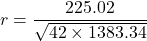

 , showing a strong positive linear correlation between study hours and exam scores.
The Pearson Correlation Coefficient is by definition a number between -1 and 1. Its sign will imply a positive or negative correlation. The closer it is to  the more it will be perfect. The closer to 0, the weaker (or no correlation) there is between the variables.
| Value of Coefficient () |
Geometric Interpretation / Strength |
|---|---|
 |
Perfect positive linear correlation |
 |
Strong positive linear correlation |
 |
Moderate positive linear correlation |
 |
Weak positive linear correlation |
 |
No linear correlation (random scatter or non-linear trend) |
 |
Weak negative linear correlation |
 |
Moderate negative linear correlation |
 |
Strong negative linear correlation |
 |
Perfect negative linear correlation |
Line of Best Fit, Interpolation and Extrapolation
If the correlation between two variables is strong enough and linear, we can draw what is called a line of best fit to illustrate the relationship. We draw a line of best fit by eye, so it will vary from person to person. Given two linearly strongly correlated variables and , we can draw the line of best fit as follows:
- Calculate the means of and , which we denote and .
- Locate the mean point
 on the scatter diagram.
- Draw a line through the mean point which fits the trend of the data, so that about the same number of data points are above the line as below it.
This final step makes the line of best fit somewhat subjective. People might rotate the line higher or lower based on what they perceive is a symmetric distribution of the points. The Pearson Correlation Coefficient aims to remove that subjectivity. Similarly, we will see how an objective line can be obtained.
Take our first example:
| Day | A | B | C | D | E | F | G | H | I | J | K | L |
|---|---|---|---|---|---|---|---|---|---|---|---|---|
| Temperature (, °C) |
11 | 15 | 16 | 19 | 13 | 20 | 12 | 10 | 21 | 17 | 14 | 14 |
| Revenue (, EUR) |
22 | 31 | 25 | 42 | 24 | 48 | 16 | 12 | 55 | 36 | 20 | 26 |
The scatter plot with the line of best fit is:
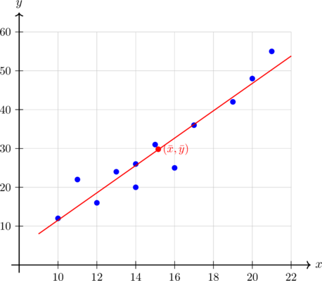
We see that the data seems to fit a line well in this case. We can use that line to understand values that are not on our table. The lowest point  and the highest point
 are sometimes referred to as lower and upper poles respectively. Whenever we use the line of best fit to predict a value between these two poles, we are doing an interpolation. A prediction outside these values is called an extrapolation.
Using the calculator, we can obtain the equation of the line of best fit and use it to make predictions, which we will do in our next page.
Exercises
Analyse the six scatter plots displayed below. For each plot, describe the type and strength of linear correlation (e.g. strong positive, moderate negative, weak positive, or no correlation) based entirely on its visual layout.


Match each of the following six Pearson correlation coefficients () to its corresponding scatter plot based entirely on the direction and strength of the point trends:
 ,
 ,
 ,
 ,
 ,


A hardware testing laboratory monitors how the internal storage size (, in GB) of six newly designed smartwatches affects their operational standby battery life (, in hours). The data collected is recorded in the table below:
| Device | A | B | C | D | E | F |
|---|---|---|---|---|---|---|
| Storage (, GB) |
16 | 32 | 64 | 128 | 256 | 512 |
| Battery life (, hours) |
72 | 68 | 65 | 58 | 52 | 40 |
- 1. Draw a scatter plot for this dataset.
- 2. Calculate Pearson’s correlation coefficient ().
- 3. Describe the type and strength of correlation based on the coefficient.
- 4. Is it realistic to expect this trend to maintain the same behaviour for significantly larger storage values (e.g. 2048 GB)?
An agricultural facility tracks how adding organic nutrient fertiliser fluid (, in mL per litre) impacts the net mass harvest yield (, in kg per square metre) of vertical greenhouse tomato crops across six test quadrants:
| Quadrant | 1 | 2 | 3 | 4 | 5 | 6 |
|---|---|---|---|---|---|---|
| Nutrient (, mL/L) |
5 | 10 | 15 | 20 | 25 | 30 |
| Yield (, kg/m²) |
14 | 22 | 29 | 35 | 44 | 50 |
- 1. Construct a scatter plot for this dataset.
- 2. Calculate Pearson’s correlation coefficient () for this dataset.
- 3. Describe the correlation between the variables.
- 4. Is it realistic to expect this behavior to continue linearly for much larger nutrient inputs?
An environmental study monitors the altitude (, in hundreds of metres) and the corresponding air temperature (, in °C) across six mountain base stations:
| Station | 1 | 2 | 3 | 4 | 5 | 6 |
|---|---|---|---|---|---|---|
| Altitude () |
2 | 5 | 8 | 11 | 14 | 17 |
| Temperature () |
24 | 22 | 17 | 13 | 11 | 3 |
- 1. Draw a scatter plot for this dataset.
- 2. Find the coordinates of the mean point
 .
- 3. Draw a line of best fit for the data set.
An engineering team tracks the runtime (, in weeks) of a heavy factory drill against the physical wear depth (, in mm) recorded on its primary gear tooth profile:
| Gear | 1 | 2 | 3 | 4 | 5 | 6 |
|---|---|---|---|---|---|---|
| Runtime () |
3 | 6 | 9 | 12 | 15 | 18 |
| Wear Depth () |
8 | 14 | 23 | 29 | 38 | 44 |
- 1. Construct a scatter plot for this data.
- 2. Find the coordinates of the mean point .
- 3. Draw the line of best fit.