When we look at the graph of a function, there are sometimes moments where the function reaches a high point or a low point. These are called extreme points. A high point is called a maximum, while a low point is called a minimum. These are examples of extreme points.
At these points, the graph often changes direction. For example, a graph may be increasing before reaching a maximum and then decreasing afterwards. Similarly, it may be decreasing before reaching a minimum and then increasing afterwards. At the very top or bottom of the curve, the tangent line is usually horizontal, which means that its slope is zero.
This connects directly to the first derivative. Since the first derivative gives us the slope of the tangent, an extreme point can often be found by looking for where the first derivative is equal to zero. In other words, we solve to find possible maximum and minimum points, and then investigate what happens around these points to decide whether they are actually maxima or minima.
The important idea is that extreme points are places where a function reaches a local high or low value, and the first derivative helps us find them.
Optional Background – Drawing a Sign Diagram
This is generally less relevant in 3 periods and although it will become relevant below, there are other ways to circumvent having to learn this. However, personally, understanding this gives a seamless way to understand an important point in the theory below (finding extreme points).
Look at the graph of the function  .
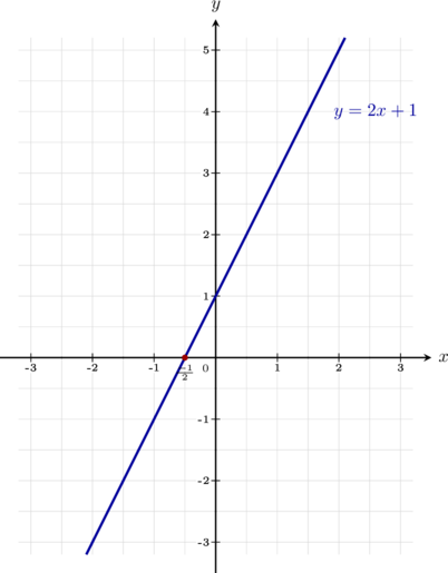
Drawing graphs can be tedious. A sign diagram attempts to eliminate the tedious part by focusing only on three things: where the function is positive, where it is negative, and where it is zero. Therefore, we care to first find where the function is 0. We locate those points on a number line, and check in each section if you function is positive or negative by replacing an appropriate value for  .

We know that the line is negative before  and positive afterwards from looking at the graph. Without the graph, we can just replace a value of that is less than
 for the left section and a value that is more than for the right section.
For example: if  we have
 which is negative. On the other hand, if
 , we have
 which is positive. Exactly as expected. That is, it is much easier and faster to draw a sign diagram that it is a graph.
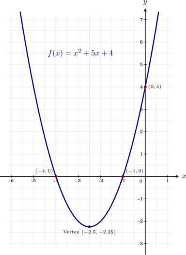
Example: Determine the signs of the quadratic function  and construct its corresponding sign diagram.
 . We look for two integers that multiply to give the constant term (
 ) and add up to give the coefficient of the middle term (
 ). These numbers are
 and




 and
 . These values partition the number line into three separate test intervals.
 ) is positive, the parabola opens upwards. This means the function outputs are negative between the two roots and positive outside of them. We can also verify this by evaluating sample test numbers:
 (test
 ):

 (test
 ):

 (test
 ):


If we wanted to look at the graph of this function, we know it is:
The Role of the Derivative
We have seen already the link between the tangent line and the first derivative. We can use the derivative to understand facts about our function using the following criteria:
Theorem (Local Monotonicity and Tangent Slopes): The connection between a function’s directional behaviour and its derivative at a given point is established through the geometric profile of its tangent line:
- Positive Derivative (
 ): The slope of the tangent line is positive, meaning the tangent line tilts upwards from left to right. Consequently, the function is locally increasing at that point.
- Negative Derivative (
 ): The slope of the tangent line is negative, meaning the tangent line tilts downwards from left to right. Consequently, the function is locally decreasing at that point.
Let us see how we use this theory.
Example: Determine the signs of the quadratic function and construct its corresponding sign diagram.
The next example is just to show how when the derivative is a quadratic function (which is harder than something linear), the main idea/method does not change.
Example: Determine where the cubic function  is locally increasing or decreasing by studying the sign of the derivative.


 .

 or
 (which can be written as
 ), the derivative is positive (
 (which can be written as
 ), the derivative is negative (
 and decreasing on
 .
As you can see, there are a few ways to write our conclusions. In the example above we said  , which can also be written as
 , or described with words by saying “all numbers between -1 and 1, not including these”.
Finding Extreme Points
The claim above concerns the sign of the derivative. That is, if  or
 we get an appropriate conclusion. What about when
 ? That is the next point we are studying.
Definition (Stationary Point): Let  be a differentiable function and
 a point in its domain. is called a stationary point if:

- : An interior point within the domain of the function where the first derivative vanishes.
- Geometric Meaning: The slope of the curve becomes flat, representing a temporary or permanent pause in the function’s vertical growth or decay.
- Classifications: Stationary points can be further categorized as local maxima, local minima, or horizontal inflection points.
From this concept of stationary points, we get the following definition:
Definition (Local Extreme Points): Let be a real-valued function and a point in an open interval within its domain. is called a local extreme point if it satisfies one of the following conditions:

- Local Maximum: A point where
 for all in a small surrounding interval, geometrically forming a local peak on the curve.
- Local Minimum: A point where
 for all in a small surrounding interval, geometrically forming a local trough on the curve.
- Necessary Condition: If is differentiable at an interior extreme point , then it must also be a stationary point where
 .
Finally, we finish the claim we began this page with by giving the real object of our study:
Theorem (The First Derivative Test for Local Extrema): At a stationary point where , the tangent line is horizontal. The geometric behaviour of the tangent lines around this point determines whether it is a local maximum or minimum:
- From Positive to Negative: If the derivative changes from positive to negative across , the tangent lines transition from tilting upwards to tilting downwards. The function goes from increasing to decreasing, creating a peak or a local maximum.
- From Negative to Positive: If the derivative changes from negative to positive across , the tangent lines transition from tilting downwards to tilting upwards. The function goes from decreasing to increasing, creating a valley or a local minimum.
In simpler terms, if before  , then the function was increasing before . When it changes to after the point , then it is decreasing. That is, the function increased until the point and then decreased, so is by definition a maximum. The argument for the minimum works analogously.
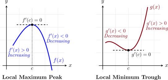
These special points are referred to as local extrema. We talk about them locally because, on the whole, a graph could have many local maxima or minima but globally they cannot all be maxima/minima unless they are equal. An example of this is the cosine and sine functions, they are periodic and their maximum value is 1 and minimum value is -1.
To find the extreme points of a function , we follow these steps:
- Find
 .
- Solve the equation .
- Draw a sign diagram of and locate all the solutions from the previous step and points of discontinuity of
 on it increasingly.
- Study the sign of the function before, after, and in between every one of those points. This will allow you to conclude the behaviour of
 .
- Conclude which points (if any) are extreme.
Example: Find and classify all local extreme points of the quadratic function  .


 .
 across the stationary point to deduce the corresponding changes in the behavior of the main function

 -coordinate:

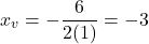
 , the single local extreme point matches the vertex of its parabola. We can calculate the
 :
 back into the original function yields
 , giving the vertex coordinates
 . Because the leading coefficient (
 .
Let us now see an example where the derivative ends up being a quadratic function, i.e.: where our original function is cubic. This is just to give a new example where we cannot cheat out the answer by using the vertex.
Example: Find and classify all local extreme points of the cubic function  .

 , and factorise the remaining quadratic equation:


 across each stationary point to deduce the corresponding changes in the behavior of the main function
 , this point is a local minimum.


 and the local minimum point is located at
 .
Second Derivative Test
This is a test that requires us to first find the second derivative, so we begin by defining it:
Definition (Second Derivative): The second derivative of a function is simply the derivative of its first derivative . It represents the rate of change of the slope of the original function and is denoted as  :

We call it the second derivative because we are differentiating the original function twice.
Example: Find the second derivative of the polynomial function defined by  .




 .
In order to conclude that a point  is a local maximum, we need three conditions:
 , i.e.: the tangent line at that point is parallel to the -axis.
- for
 , i.e.: the function increases until that point.
- for
 , i.e.: the function decreases after that point.
Similarly, for to be a local minimum, we require:
- , i.e.: the tangent line at that point is parallel to the -axis.
- for , i.e.: the function decreases until that point.
- for , i.e.: the function increases after that point.
We have done this by drawing a sign diagram of , thus making the second derivative irrelevant in this process. However, instead of doing a sign diagram for we can use the second derivative to draw the same conclusions, as the next claim will show.
Claim (The Second Derivative Test): Let be a function such that its first derivative equals zero at a critical point ( ), and its second derivative is continuous in an open interval around . The classification of this stationary point is determined by the sign of the second derivative at that location:
- If
 , then has a local minimum at .
- If
 , then has a local maximum at .
- If
 , the test is inconclusive (the point could be a local maximum, local minimum, or a stationary inflection point).
 . Since we are given that
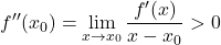
 must also be positive for all
 ), the denominator is negative (
 ). To keep the quotient positive, the numerator must also be negative, meaning
 ), the denominator is positive (
 ). To keep the quotient positive, the numerator must also be positive, meaning
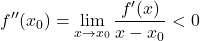
To use this in an example, we have:
Example: Find and classify all local extreme points of the cubic function  by using the second derivative test.


 , and factor the quadratic expression to solve for the critical inputs:



 , the curve is concave down at this point (frowning shape). A horizontal tangent line on a concave down curve means
 :

 , the curve is concave up at this point (smiling shape). A horizontal tangent line on a concave up curve means


 and the local minimum point is located at
 .
Exercises
For each of the following four functions, find the coordinates of all stationary points. Differentiate the function to find , solve the equation  to identify the stationary -values, and evaluate at those points to get the full coordinate pairs.



For each of the following real-valued functions, calculate the first derivative, find all stationary points, and classify them as local maxima, local minima, or non-extremes using a sign diagram.



Calculate the second derivative with respect to for each of the following functions. First evaluate using standard rules, and then differentiate a second time to determine . Simplify your answers where possible.



Find the coordinates of all stationary points for each of the following 3 functions and classify them as local maxima or local minima by applying the second derivative test instead of a sign diagram:
- Quadratic Function:

- Cubic Function A:

- Cubic Function B:
