Having defined what a discrete random variable is, we move on to concepts that were first discussed in Statistics in S4 and S5 except defined with a probabilistic approach.
Expectation
The expectation (or expected value) of a discrete random variable is the weighted average of all its possible values, where each value is weighted according to its probability.
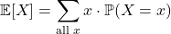
Definition (Expected Value of a Discrete Random Variable): The Expected Value (also called the expectation or mean) of a discrete random variable  is the long-run theoretical average outcome if the underlying experiment were repeated an infinite number of times. It is a weighted average where each possible value of is multiplied by its corresponding probability from the PDF, denoted by
 or
 :

That is, we multiply each  (each value our variable can get) by its respective
 (the probability of being that value) and add the results. We know that if we toss a coin twice, we expect to see one Heads, let us show this:
Example: A fair coin is tossed twice. Let the discrete random variable represent the total number of times the coin lands on Heads. Prove mathematically that the expected value of is exactly  (
 ).
 . We first lay out the distribution values in a clean table.
 , the probability density function for the number of Heads is:

 by its corresponding column probability
 and sum the products together:



Of course, the expectation of a discrete random variable can be found in any case, whether we know the context or not:
Example: A discrete random variable has the probability distribution defined by the following Probability Density Function (PDF):

Calculate the expected value for this discrete random variable.








 .
We can also use a given expectation to find missing probabilities:
Example: A discrete random variable has the probability distribution shown in the table below, where two probabilities are missing and represented by the variables  and
 .

Given that the expected value of the random variable is  , set up a system of linear equations to solve for the missing probabilities and .











 back into Equation 1 to find


 and
 , confirming a mathematically sound distribution layout.
Properties of the Expectation
Instead of just being given a discrete random variable , we could discuss the expectation when a function is applied to , i.e.:  .
Definition (Expected Value of a Function of a Random Variable): Let be a discrete random variable that takes on a finite set of distinct real values  with corresponding probabilities
 (where
 ). If
 is a real-valued function applied to , the expected value of , denoted by
 , is the weighted average of the values that the function can take, given by the formula:
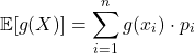
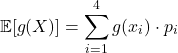
This property is highly powerful because it states that to find the expectation of the transformed variable , you do not need to first derive the actual Probability Density Function (PDF) of . Instead, you can calculate it directly by applying the function  directly to the original support values of and multiplying down the original columns of your probability distribution.
Example: A discrete random variable has the probability distribution defined by the following Probability Density Function (PDF):

Let  . Calculate the expected value .
 :
 :

 :

 :

 :





 is exactly
 .
Finally, below are two simple but powerful properties that will allow you to calculate expectation more easily.
Claim (Properties of Expectation): Let be a discrete random variable with a finite expected value , and let  ,
 , and
 be any fixed real constants. The expectation operator satisfies the following two fundamental properties:
- Expectation of a Constant: The expected value of any fixed constant value is exactly equal to the constant itself:

- Linear Transformation of Expectation (Linearity): The expected value of a linear combination scales and shifts predictably according to the linear transformation parameters:

 , and
 everywhere else. Applying the discrete expectation definition:





 is exactly the definitive definition of the expected value,
 is the sum of all probabilities over the complete sample space support, which must equal

The linearity of expectation is a particularly useful property for discussing fair games.
Definition (Fair Game): A game or investment scenario is called fair if its expected earning is equal to zero. If the discrete random variable represents the net financial profit or loss resulting from playing the game, it is fair if and only if:

A fair game represents a situation of equilibrium. It implies that in the long run, over a vast number of repetitions, a player will theoretically neither win nor lose any money. If  , the game carries a positive expected value favouring the player; if
 , it carries a negative expected value favouring the house.
Example: At a carnival game, a player pays a non-refundable ticket price of  W
 12.
 0).
Tasks:
1. Let represent the player’s net profit. Construct the PDF table for and calculate to determine if the game is mathematically fair.
2. Use the linearity of expectation to find what the entry ticket cost should be changed to so that the carnival game becomes perfectly fair.
 and subtracting the initial ticket price of
 (
 ). Let’s find the net profit values and their probabilities:
 ): Net profit is

 ): Net profit is

 ): Net profit is

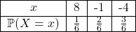


 , the game is not fair. On average, the player loses
 c
 X_{\text{new}} = W – c
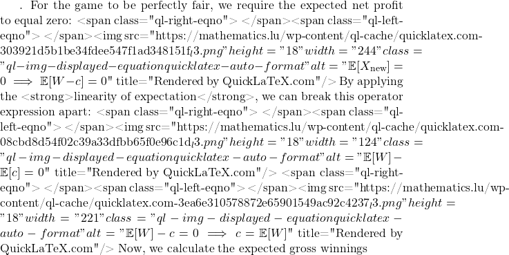
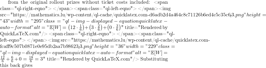
 3 for the game to be mathematically fair.
Variance and its Properties
The variance of a discrete random variable measures how spread out its possible values are around the expected value (mean). A small variance means the values are clustered close to the mean. A large variance means the values are more spread out.
Definition (Variance of a Discrete Random Variable): The Variance of a discrete random variable measures the dispersion or spread of the probability distribution around its mean . It is defined as the expected value of the squared deviations from the mean. It is denoted by  or
 and calculated using the formula:

There is an alternative way to calculate the variance of a discrete random variable, as the claim below will show:
Claim (Alternative Variance Formula): For any discrete random variable with a finite mean  , the variance can be computed using the following identity, often referred to as the computational or shortcut formula:





 is the expected value of
 , which is written as
 .



The following example will show how each of the formulas above can be used to find  :
Example: A discrete random variable has the probability distribution defined by the following Probability Density Function (PDF):

Calculate the variance using two different methods to prove they are equivalent:
1. The Definitional Formula: 
2. The Computational Formula: 
 first, so we compute that as our shared baseline step:


 ), square it, multiply it by its column probability, and sum them up:

 :

 :

 :

 :






 and
 into the computational formula:


 .
In general, you are allowed to use whichever formula you prefer.
We finish with a simple property of the variance:
Claim (Properties of Variance): Let be a discrete random variable with a finite variance , and let , , and be any fixed real constants. The variance operator satisfies the following two fundamental properties:
- Variance of a Constant: The variance of any fixed constant value is exactly zero:

- Linear Transformation of Variance (Linearity): The variance of the linear combination
 scales by the square of the multiplicative constant:

 . Substituting this into the definitional formula for variance yields:

 ):




 is a constant multiplier, we pull it completely out of the expectation operator:

Below is an example of how we use this property.
Example: A discrete random variable representing daily sales at a retail store has a known variance of  . The net daily profit,
 , is modeled as a linear transformation of sales given by the equation:

Calculate the variance of the net daily profit,  , by applying the properties of the linearity of variance.
 , we use the theorem for the linear transformation of variance:





 . Notice that the constant subtraction of
 has zero effect on the spread of the distribution, while the scaling multiplier of
 affects the variance by a squared factor of
 .
Standard Deviation
Our final concept is that of standard deviation, you have seen this in statistics in S5 but here we are redefining it using probability language.
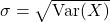
Definition (Standard Deviation of a Discrete Random Variable): The Standard Deviation of a discrete random variable is a metric that quantifies the absolute amount of dispersion, variation, or spread in a probability distribution. It is denoted by  or
 , and is expressed by the formula:

The standard deviation acts as a baseline measure for how far away a typical outcome falls from the mean ().
Example: A discrete random variable has a probability distribution defined by the following Probability Density Function (PDF):

Find the standard deviation for this random variable. Round your final answer to four decimal places.
 .


 . First, let’s find the expected value of the squares,



 and
 into the variance formula:



 . This tells us that the typical distance of the outcomes from the theoretical center mean of
 is exactly
Exercises
A discrete random variable has the probability distribution listed in the table below:

Evaluate this probability distribution by calculating the following key summary metrics:
- The expected value .
- The variance using either the definitional or computational formula.
- The standard deviation .
The Probability Density Function (PDF) of a discrete random variable is given by the tracking matrix below:

Determine the fundamental statistical dispersion properties of the distribution:
- The theoretical long-run average mean .
- The measurement of variance .
- The standard deviation
 ,.
A discrete random variable distributes its probability according to the following fraction baseline:

Evaluate this rational distribution using fraction calculations until the final decimal conversions:
- The expected value .
- The variance .
- The standard deviation .
The complete Probability Density Function (PDF) of a discrete random variable is provided in the tracking matrix below. Two fractional probability spaces are unknown and defined as parameters and :

Given that the expected value is exactly  , formulate and solve a system of linear equations to determine the value of the missing fractions and .
A discrete random variable has the probability distribution layout detailed below. Two probability metrics are missing and labeled as variables and :

Given that the expected value of this distribution is  , construct a system of linear equations using the total normalization property and the mean parameter to calculate the exact values of and .
A charity fundraising event features a game using a fair spinner divided into 8 equal sectors. It costs exactly $5 to play one round. The gross cash rewards based on where the spinner stops are structured as follows:
- Landing on Sector 1: The house pays the player $24.
- Landing on Sectors 2 or 3: The house pays the player $8.
- Landing on any other sector: The player receives nothing ($0).
Question: Should you play this game if your primary goal is to turn a net financial profit over a large number of attempts? Justify your decision explicitly by calculating the expected net profit of a round.
A game of chance involves drawing a single card at random from a standard deck of 52 playing cards. A participant currently pays an entry fee of $3 per round. The payout structure based on the suit drawn is defined below:
- Drawing an Ace of Spades: The player wins a cash prize of $50.
- Drawing any other Spade: The player wins a cash prize of $6.
- Drawing any other suit: The player receives nothing ($0).
- Construct the Probability Density Function (PDF) table for the player’s net profit and calculate to determine if the game is currently fair.
- Apply the linearity property of expectation to find what the entry cost should be changed to so that the card game becomes perfectly fair (
 ).
Let be a discrete random variable with a finite standard deviation , and let  be fixed constants.
Show that:

Hint: Use the linearity of the variance.