The final topic of the year is binomial variables. These are a type of discrete random variable. In order to define these, we need to put into context the theory we have discussed in the last couple of pages.
Bernoulli Variables
These are a special type of variable focused on a simple concept: we define a success and a failure for an instance of an experiment and give them the values 1 and 0 respectively. It is the simplest type of discrete random variable.
Definition (Bernoulli Random Variable): A Bernoulli random variable models a single trial or experiment that has exactly two possible outcomes: a “Success” (mapped to numerical value  ) or a “Failure” (mapped to numerical value
 ). It depends on a single parameter
 , which represents the probability of a success.
Probability Density Function (PDF):
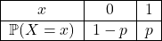
This we symbolise as  or
 . This means that
 has Bernoulli distribution and the probability of success is .
Now we can see how a few simple examples we have discussed were actually Bernoulli variables.
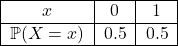
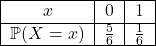
Example: Show how a single coin toss and rolling a standard six-sided die once can be classified and structured as Bernoulli random variables.
 )
 )
 . Its PDF table is structured as:
 distinct outcomes, but we can transform it into a Bernoulli variable by defining a specific condition, such as “rolling a 6”:
 )
 or
 )
 . Its PDF table is structured as:
As you can see, Bernoulli variables are nothing special per se, but they help us define a more interesting type of variable.
Properties of a Bernoulli Variable
Once we know that a variable has Bernoulli distribution (another way of saying it is a Bernoulli variable), we can understand immediately what its expectation, variance, and standard deviation are without having to do the entire work as in the previous page. The following claim will show these formulas:
Claim (Parameters of a Bernoulli Variable): Let be a Bernoulli random variable with success parameter , where  . The expected value
 , variance
 , and standard deviation
 as a function of are given by the following equations:



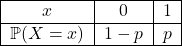
 across the two valid states:



 . First, we compute the expected value of the squared variable,
 , by applying the function definition:



 and





That is, once we know , the expectation, variance, and standard deviation will always be predetermined.
Example: In a manufacturing plant, a quality control audit shows that  of the manufactured parts are structurally defective. A single part is selected completely at random. Let the random variable be a Bernoulli variable where a “Success” (
 ) represents selecting a defective part, and a “Failure” (
 ) represents selecting a non-defective part. Calculate the expected value , the variance , and the standard deviation for this variable.


 . Substituting our value for



 ,
 , and
 .
Binomial Distribution and Properties
When many Bernoulli variables are taken together, they create what is known as a Bernoulli process. Let  be
 Bernoulli variables, all independent, and with probability of success . Then, the variable
 is a Binomial variable.
Definition (Binomial Random Variable): Let a Bernoulli process consist of a sequence of independent and identically distributed (i.i.d.) Bernoulli variables. For every  , the probability of obtaining a “Success” () in
 is and the probability of a “Failure” () be
 . A variable is a Binomial random variable, denoted by
 . It tracks the cumulative number of successes across these independent Bernoulli trials.
Probability Density Function:
The probability of obtaining exactly  successes in trials is given by multiplying the number of ways to arrange the successes by the joint probability of achieving that specific count of successes and failures:

Where 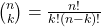 represents the binomial coefficient counting the combinations of branches containing exactly
 successes.
The reason for the formula above is the following: If you want successes out of trials, you need  for the successes,
 since the rest must be failures, and the factor
 shows the number of ways we can choose variables to be successes.
Our first goal is to be able to recognise Binomial variables. In reality, you have already seen examples of this.
Example: Show how the following three separate experiments can be modeled as Binomial random variables. For each case, explicitly justify why the conditions of a Bernoulli process are satisfied and identify the parameters and .
- Experiment 1: Tossing a fair coin 10 times and counting the total number of Heads.
- Experiment 2: Rolling a fair six-sided die 15 times and counting how many times it lands on a 5.
- Experiment 3: Selecting 20 items at random from a factory production line where 4% of items are defective, and counting the total number of defective items.
 is the Bernoulli trial of the first coin toss,
 is the trial for the second coin toss, and so on. Because the coin is fair, the probability of rolling Heads remains a constant 0.5 for every single flip. Furthermore, the coin tosses are independent.
 , and probability of success
 ).
 ) as a “Failure”. For a standard fair die, the chance of hitting a 5 is
 for each throw. Rolls are independent.
 is a binomial variable.
 , and probability of success
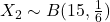 ).
 , and probability of success
 (
 ).
Much like the Bernoulli variables, we have a fixed expectation, variance, and standard deviation as a function of and .
Theorem (Parameters of a Binomial Random Variable): Let be a Binomial random variable tracking the total number of successes across independent and identically distributed (i.i.d.) Bernoulli trials, each having a constant success probability . The expected value , variance , and standard deviation  are given by:



 . Recall that for any individual Bernoulli trial
 and
 .





This explains the intuition people typically have behind coin tosses. If you toss 20 fair coins, you expect to see 10 heads. This is because if is the number of times the coin lands on Heads, then  with
 and
 . The expectation is therefore
 .
Examples of Binomial Variables
The examples below will all include probability calculations as well as finding the expectation, variance, and standard deviation of binomial variables in different contexts.
Example (Coin Tosses): A fair coin is tossed  times in succession. Let the random variable represent the total number of times the coin lands on Heads.
- Calculate the exact probability that the coin lands on Heads exactly
 times (
 ).
- Calculate the exact probability that the coin lands on Heads at least
 times (
 ).
- Find the expected value , variance , and standard deviation of this distribution.
 and a constant success probability
 ).
 :

 and
 are mutually exclusive outcomes:







Let us move on to another example, now with dice, just to cover the two classical examples you have seen in simple experiments.
Example (Die Rolls): A fair six-sided die is rolled times. Let the random variable represent the total number of times the die lands on a  .
- Calculate the exact probability that the die lands on a exactly time (
 ).
- Calculate the exact probability that the die lands on a at least times (
 ).
- Find the expected value , variance , and standard deviation of this distribution. Round to four decimal places.
 trials and a constant success probability
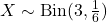 ).
 and
 :

 and







Another typical example is counting the number of defective objects created in a manufacturing process.
Example (Factory Production): A factory production line creates microchips where  are known to be defective. A quality analyst randomly selects a sample of microchips. Let the random variable represent the total number of defective microchips in the sample.
- Calculate the exact probability that the sample contains exactly defective microchips (
 ).
- Calculate the exact probability that the sample contains at least defective microchip (
 ).
- Find the expected value , variance , and standard deviation of this distribution. Round to four decimal places.
 items and a constant defect success probability
 (
 ).
 successes occur:

 ), evaluate this efficiently using the complement rule:





The next example is meant to show how an everyday situation can be modelled using binomial variables.
Example (Multiple Choice Guessing): A student answers a short multiple-choice quiz consisting of questions completely by random guessing. Each question has options, with only one correct answer. Let the random variable represent the number of questions answered correctly.
- Calculate the exact probability that the student guesses exactly questions correctly (
 ).
- Calculate the exact probability that the student gets a passing mark of at least questions correctly (
 ).
- Find the expected value , variance , and standard deviation of this distribution. Round to four decimal places.
 per question (
 ).
 successes and
 failures:

 :






Exercises
For each of the 8 scenarios described below, determine whether the random variable is a Binomial random variable.
• If it is Binomial, explicitly state the parameters and .
• If it is not Binomial, briefly explain which core condition of a Bernoulli process is violated.
- Scenario A: A standard fair coin is flipped until the first time it lands on Heads. Let represent the total number of flips required.
- Scenario B: A student randomly guesses the answers on a 20-question multiple-choice exam where each question has 5 options (only one correct). Let represent the total number of correct answers.
- Scenario C: Five cards are drawn sequentially from a standard, well-shuffled 52-card deck without replacing the card back into the deck between draws. Let represent the total number of Hearts collected.
- Scenario D: Five cards are drawn sequentially from a standard, well-shuffled 52-card deck, but each card is completely replaced and the deck reshuffled before the next draw. Let represent the total number of Hearts collected.
- Scenario E: A basketball player with an 80% free-throw average shoots 10 free throws. Let represent the total number of successful free throws made, assuming each shot is independent.
- Scenario F: A fair six-sided die is rolled 50 times. Let represent the total number of times the die lands on either an even number or a 5.
- Scenario G: A box contains 3 red balls, 4 blue balls, and 5 green balls. A ball is drawn at random, its color is recorded, and it is placed back in the box. This process is repeated 12 times. Let track the total number of times a blue ball or a green ball is drawn.
- Scenario H: A commuter drives through 4 independent traffic lights on their way to work. The first light has a 40% chance of being red, the second has a 50% chance, the third a 30% chance, and the fourth a 60% chance. Let track the total number of red lights encountered.
A electronics hardware manufacturer tracks component reliability. Records show that 20% of circuit boards fail a rigorous stress test. A quality inspector selects a random sample of circuit boards. Let the random variable represent the number of circuit boards that fail the stress test.
- Calculate the exact probability that exactly boards fail the stress test.
- Calculate the exact probability that at least boards fail the stress test.
- Find the expected value , variance , and standard deviation
 of this distribution. Round your final values to two decimal places.
An analytics team monitors a software support hotline. Historical metrics reveal that  (
 ) of incoming calls are successfully resolved by the first tier of support. A supervisor randomly selects a batch of
 calls to audit. Let the random variable track the number of calls resolved by the first tier.
- Explain why is a binomial variable and state its parameters.
- Calculate the exact probability that exactly
 calls are successfully resolved.
- Calculate the exact probability that at least
 calls are successfully resolved.
- Find the expected value , variance , and standard deviation of this distribution. Round your final values to two decimal places.
Ecologists tag a large population of sea turtles in a marine reserve. Exactly  of the regional population has been successfully fitted with tracking tags. Field scientists spot sea turtles at random during a dive. Let the random variable represent the number of spotted turtles carrying a tracking tag.
- Calculate the exact probability that exactly turtle carries a tracking tag.
- Calculate the exact probability that at least turtles carry a tracking tag.
- Find the expected value , variance , and standard deviation of this distribution. Round your final values to two decimal places.
An e-commerce company tracks dispatch delays. Operations metrics confirm that only 10% of parcels encounter shipping delays. A courier depot isolates a random selection of parcels for tracking. Let the random variable represent the number of parcels encountering a shipping delay.
- Explain why is a binomial variable and state its parameters.
- Calculate the exact probability that exactly parcels encounter a shipping delay.
- Find the expected value , variance , and standard deviation of this distribution. Round your final values to two decimal places.