Previous Knowledge Required: Basic limit calculation and properties of functions (S6).
This section in S7 mainly discusses two specific topics: Indeterminate forms of limits and Oblique Asymptotes. The main properties of functions discussed in S6 are:
- Domain of definition
- Range
- Asymptotes
- Extreme Points
- Increasing/Decreasing behaviour of functions
- Inflection Points
- Convexity and Concavity
These properties should be studied to an extended list of functions as:





 for
for 


- Polynomials of degree at most 3
 where
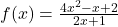
where  are polynomials of degree at most 2.
For now, this page will focus on the main two topics and at future could be expanded to do a study on this extended list of functions.
Indeterminate Forms of Limits
You will have studied in S6 the following rules for calculating limits:
Claim (Basic Arithmetic Limit Rules): Let  be a fixed, non-zero real constant (
 ). The behavior of foundational quotient, product, and reciprocal limits involving infinities and zeros evaluates according to specific fixed structural laws.
![\[\frac{\pm\infty}{L} = \pm\infty \quad \text{and} \quad \frac{L}{0} = \pm\infty\]](https://mathematics.lu/wp-content/ql-cache/quicklatex.com-d55731b1fa31f8978a314a96e1b7f6d3_l3.png "Rendered by QuickLaTeX.com")
![\[\frac{\infty}{L > 0} = \infty, \quad \frac{\infty}{L < 0} = -\infty, \quad \frac{-\infty}{L > 0} = -\infty, \quad \frac{-\infty}{L < 0} = \infty\]](https://mathematics.lu/wp-content/ql-cache/quicklatex.com-55d680bfee349106224d2561ae125e9d_l3.png "Rendered by QuickLaTeX.com")
![\[\frac{L > 0}{0^+} = \infty, \quad \frac{L > 0}{0^-} = -\infty, \quad \frac{L < 0}{0^+} = -\infty, \quad \frac{L < 0}{0^-} = \infty\]](https://mathematics.lu/wp-content/ql-cache/quicklatex.com-31a5478786eae4eac61ac455dbf53b66_l3.png "Rendered by QuickLaTeX.com")
![\[\frac{L}{\infty} = 0, \quad \frac{L}{-\infty} = 0\]](https://mathematics.lu/wp-content/ql-cache/quicklatex.com-fd0d060806537c8b1f3298a99b0b8870_l3.png "Rendered by QuickLaTeX.com")
![\[(\pm\infty) \cdot (L > 0) = \pm\infty, \quad (\pm\infty) \cdot (L < 0) = \mp\infty, \quad (\infty) + (\infty) = \infty, \quad (-\infty) + (-\infty) = -\infty\]](https://mathematics.lu/wp-content/ql-cache/quicklatex.com-ff6bcc197a8cd3266a7b30743bdb0561_l3.png "Rendered by QuickLaTeX.com")
However, limits of the form  and
and  we are told that they depend on the situation. For example.
Example: Evaluate the limit of the rational function as  approaches positive infinity:
![\[\lim_{x \to \infty} \frac{2x^2 - 3x + 1}{5x + 4}\]](https://mathematics.lu/wp-content/ql-cache/quicklatex.com-01d6d7f838cd421679122c87976313e5_l3.png "Rendered by QuickLaTeX.com")
 into both the quadratic numerator and linear denominator yields an indeterminate ratio:
![\[\frac{\infty}{\infty}\]](https://mathematics.lu/wp-content/ql-cache/quicklatex.com-9e8511152de04d9fccca948b55f3f70c_l3.png "Rendered by QuickLaTeX.com")
![\[\lim_{x \to \infty} \frac{\frac{2x^2}{x} - \frac{3x}{x} + \frac{1}{x}}{\frac{5x}{x} + \frac{4}{x}} = \lim_{x \to \infty} \frac{2x - 3 + \frac{1}{x}}{5 + \frac{4}{x}}\]](https://mathematics.lu/wp-content/ql-cache/quicklatex.com-7bb9fb879d11f90604fd2491684e4c7d_l3.png "Rendered by QuickLaTeX.com")
 and
and  approach
  . Evaluate the remaining expression components:
![\[\frac{\lim_{x \to \infty}(2x - 3 + 0)}{5 + 0} = \frac{\infty}{5}\]](https://mathematics.lu/wp-content/ql-cache/quicklatex.com-6eff71ab10617c16a5d46dd5d601651f_l3.png "Rendered by QuickLaTeX.com")
![\[\lim_{x \to \infty} \frac{2x^2 - 3x + 1}{5x + 4} = \infty\]](https://mathematics.lu/wp-content/ql-cache/quicklatex.com-b2824e452a70ad5f1aa46efe233051a5_l3.png "Rendered by QuickLaTeX.com")
Similarly, we can show the reciprocal limit going to 0. So how do we compare limits of the form:
![\[\lim_{x\to\infty}\frac{e^x}{x}\]](https://mathematics.lu/wp-content/ql-cache/quicklatex.com-51af602d4fb283649f8dbf39beb91ef4_l3.png "Rendered by QuickLaTeX.com")
You might have been told that exponential functions grow faster than linear and so the limit must be infinity. This is true, but we can show this more formally with the following theorem:
Theorem (L’Hôpital’s Rule): Let  and
and  be differentiable functions on an open interval containing
  (except possibly at itself). If
  or
or  and
and  , and if
  near , then the limit of the quotient is equal to the limit of the ratio of their derivatives, provided the limit exists or equals
  .
.
![\[\lim_{x \to c} \frac{f(x)}{g(x)} = \lim_{x \to c} \frac{f'(x)}{g'(x)}\]](https://mathematics.lu/wp-content/ql-cache/quicklatex.com-cd84b37ef85ead7fa6a0ead7b60f0b65_l3.png "Rendered by QuickLaTeX.com")
This law provides an analytical method to resolve indeterminate forms by evaluating the relative rates of change of the functions. It remains valid when approaches infinity ( ) or for one-sided limits. The rule is written a bit too formally for the required level. The idea being that the limit will not change if we differentiate each function in the fraction separately, as long as we keep having the special forms of limits
  .
.
Example: Evaluate the limit using L’Hôpital’s Rule:
![\[\lim_{x \to \infty} \frac{e^x}{x}\]](https://mathematics.lu/wp-content/ql-cache/quicklatex.com-65bf7b00ba4cde03e885c93c036bb414_l3.png "Rendered by QuickLaTeX.com")
 and the denominator
 ![\[\frac{d}{dx}[e^x] = e^x, \quad \frac{d}{dx}[x] = 1\]](https://mathematics.lu/wp-content/ql-cache/quicklatex.com-93ab693c41b6f868667fb9bdd29a9b60_l3.png "Rendered by QuickLaTeX.com")
![\[\lim_{x \to \infty} \frac{e^x}{1} = \lim_{x \to \infty} e^x = \infty\]](https://mathematics.lu/wp-content/ql-cache/quicklatex.com-93a719b0b1361065bd217703aac55591_l3.png "Rendered by QuickLaTeX.com")
![\[\lim_{x \to \infty} \frac{e^x}{x} = \infty\]](https://mathematics.lu/wp-content/ql-cache/quicklatex.com-18e9b83b8063081b79b271f86007c7ae_l3.png "Rendered by QuickLaTeX.com")
Example: Evaluate the fundamental trigonometric limit using L’Hôpital’s Rule:
![\[\lim_{x \to 0} \frac{\sin(x)}{x}\]](https://mathematics.lu/wp-content/ql-cache/quicklatex.com-9a5b9b0579e336a4b945a3ebb96afec6_l3.png "Rendered by QuickLaTeX.com")
 into the expression yields sine of zero over zero, which is an indeterminate ratio:
![\[\frac{0}{0}\]](https://mathematics.lu/wp-content/ql-cache/quicklatex.com-c53530e3c00e78129a7a1d79bb5e2483_l3.png "Rendered by QuickLaTeX.com")
![\[\frac{d}{dx}[\sin(x)] = \cos(x), \quad \frac{d}{dx}[x] = 1\]](https://mathematics.lu/wp-content/ql-cache/quicklatex.com-d4881cd59f5257d48631ad024fdf646b_l3.png "Rendered by QuickLaTeX.com")
![\[\lim_{x \to 0} \frac{\cos(x)}{1} = \frac{\cos(0)}{1} = \frac{1}{1}\]](https://mathematics.lu/wp-content/ql-cache/quicklatex.com-6fee44ec9920e29a731431aed1cdf4b0_l3.png "Rendered by QuickLaTeX.com")
![\[\lim_{x \to 0} \frac{\sin(x)}{x} = 1\]](https://mathematics.lu/wp-content/ql-cache/quicklatex.com-5de92af4c8c48fbb29669a5b6ba81b7c_l3.png "Rendered by QuickLaTeX.com")
What about a limit of the form ? We can change one of the functions so that we end up with a limit of  or
or  .
.
Example: Evaluate the indeterminate product limit using L’Hôpital’s Rule:
![\[\lim_{x \to 0^+} x \ln(x)\]](https://mathematics.lu/wp-content/ql-cache/quicklatex.com-464f215109a92ccc7e61e9ee4861d9bd_l3.png "Rendered by QuickLaTeX.com")
 and
and  , which forms an indeterminate product:
![\[0 \cdot (-\infty)\]](https://mathematics.lu/wp-content/ql-cache/quicklatex.com-4e1dc5641908505f9a8268819e96ae38_l3.png "Rendered by QuickLaTeX.com")
![\[\lim_{x \to 0^+} \frac{\ln(x)}{\frac{1}{x}} \implies \frac{-\infty}{\infty}\]](https://mathematics.lu/wp-content/ql-cache/quicklatex.com-a4a909a1c54c2445b6a4f5c164731824_l3.png "Rendered by QuickLaTeX.com")
![\[\frac{d}{dx}[\ln(x)] = \frac{1}{x}, \quad \frac{d}{dx}\left[\frac{1}{x}\right] = -\frac{1}{x^2}\]](https://mathematics.lu/wp-content/ql-cache/quicklatex.com-cae6d4ccb413d174c28b87dfb52359d8_l3.png "Rendered by QuickLaTeX.com")
![\[\lim_{x \to 0^+} \frac{\frac{1}{x}}{-\frac{1}{x^2}} = \lim_{x \to 0^+} \left( \frac{1}{x} \cdot (-x^2) \right) = \lim_{x \to 0^+} (-x)\]](https://mathematics.lu/wp-content/ql-cache/quicklatex.com-cd0d8ba8f50692ba25e959dc76a2c710_l3.png "Rendered by QuickLaTeX.com")
![\[\lim_{x \to 0^+} x \ln(x) = 0\]](https://mathematics.lu/wp-content/ql-cache/quicklatex.com-d32b1057a1f518e1eea586b9ed77b252_l3.png "Rendered by QuickLaTeX.com")
Oblique Asymptotes
You have learned in S6 that functions could have either horizontal or vertical asymptotes. There is a third type of asymptote that you study in S7 called oblique asymptotes. The idea is as follows: If you are given a rational function, that is, a quotient of two polynomials, then the behaviour as  could resemble that of a line.
If the numerator is a quadratic function, and the denominator is a linear function, it makes sense that we can somehow obtain at some point a comparable linear function. This is indeed the case as .
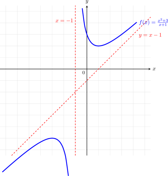
In the example above we see the vertical asymptote  and the oblique asymptote
  . In order to find the oblique asymptote, we have two methods. The first is polynomial division:
Example: Find the oblique asymptote of the rational function  using polynomial long division.
 by the denominator
  to rewrite the rational expression:
![\[\begin{array}{rll} \phantom{x+1\,} x - 1 & \text{(Quotient)} \\ x+1 \, \overline{\smash{)} \, x^2 + 0x + 3} \\ \underline{-(x^2 + x)\phantom{x+3}} \\ -x + 3 \\ \underline{-(-x - 1)} \\ 4 & \text{(Remainder)} \end{array}\]](https://mathematics.lu/wp-content/ql-cache/quicklatex.com-6cc2f44b7322e85c8ca576f81327f202_l3.png "Rendered by QuickLaTeX.com")
![\[f(x) = x - 1 + \frac{4}{x+1}\]](https://mathematics.lu/wp-content/ql-cache/quicklatex.com-abf06f7bda15cd7b3e16ac4e18282c8a_l3.png "Rendered by QuickLaTeX.com")
![\[\lim_{x \to \pm\infty} \frac{4}{x+1} = 0\]](https://mathematics.lu/wp-content/ql-cache/quicklatex.com-ecc755943663ea6c12bf2b2a240f391f_l3.png "Rendered by QuickLaTeX.com")
An alternative approach is to use the division algorithm differently. When we divide  (dividend) by
  (divisor) we are left with
  (quotient) and
  (remainder). All of these are functions of . The oblique asymptote is the and we can say:
![\[\frac{P(x)}{D(x)}=Q(x)+\frac{R(x)}{D(x)}\implies P(x)=Q(x)\cdot D(x)+R(x)\]](https://mathematics.lu/wp-content/ql-cache/quicklatex.com-69d05d84bee56b2856781e1a2c58449d_l3.png "Rendered by QuickLaTeX.com")
Using this, we can compare the coefficients of the different powers of
and understand what is. The in this formula is irrelevant.
Example: Determine the oblique asymptote of the rational function by using the method of undetermined coefficients to set up a polynomial identity.
Step 1: Set up the algebraic identity structure
Since the numerator  is a quadratic function and the denominator
  is linear, the resulting quotient must be a linear expression of the form
  , and the remainder must be a constant
  . We can relate these components using the polynomial identity:
![\[x^2 + 3 = (x + 1)(Ax + B) + C\]](https://mathematics.lu/wp-content/ql-cache/quicklatex.com-c65415463eee90f5d4ab9af8618cf042_l3.png "Rendered by QuickLaTeX.com")
Step 2: Expand and equate matching coefficients
Expand the right side of the equation and group the terms by the powers of :
![\[x^2 + 3 = Ax^2 + Bx + Ax + B + C\]](https://mathematics.lu/wp-content/ql-cache/quicklatex.com-5b25128cc561e47b0ca211c8158cb98f_l3.png "Rendered by QuickLaTeX.com")
![\[x^2 + 0x + 3 = Ax^2 + (A + B)x + (B + C)\]](https://mathematics.lu/wp-content/ql-cache/quicklatex.com-d5b43e2aec584667d4db30b5f52ae6a9_l3.png "Rendered by QuickLaTeX.com")
Compare the coefficients of identical powers of on both sides to construct a system of linear equations:
![\[\text{For } x^2: \quad A = 1\]](https://mathematics.lu/wp-content/ql-cache/quicklatex.com-1478db79d44af8ddd92185c7f96cc907_l3.png "Rendered by QuickLaTeX.com")
![\[\text{For } x^1: \quad A + B = 0 \implies 1 + B = 0 \implies B = -1\]](https://mathematics.lu/wp-content/ql-cache/quicklatex.com-df8a796a0c359b2f34584c24e1d5376c_l3.png "Rendered by QuickLaTeX.com")
![\[\text{For } x^0: \quad B + C = 3 \implies -1 + C = 3 \implies C = 4\]](https://mathematics.lu/wp-content/ql-cache/quicklatex.com-9038f5377b111551303926465574a250_l3.png "Rendered by QuickLaTeX.com")
Step 3: Analyze long-term function behavior
Substitute the solved constant values back into the structural form of the rational function:
![\[f(x) = \frac{(x + 1)(x - 1) + 4}{x + 1} = x - 1 + \frac{4}{x + 1}\]](https://mathematics.lu/wp-content/ql-cache/quicklatex.com-c1a09454a8aeb975e42061264e87a82c_l3.png "Rendered by QuickLaTeX.com")
As , the remainder component vanishes ( ). Consequently, the specific value of the constant is not relevant to determining the asymptotic trajectory.
Conclusion:
The linear quotient determines the boundary line behavior, yielding the oblique asymptote equation:  .
.
Exercises
Evaluate each of the following limits by verifying the indeterminate form or and applying L’Hôpital’s Rule. Note that one of these problems will require differentiating a second time to resolve the indeterminacy.
- 1.

- 2.
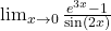
- 3.
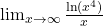
- 4.
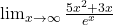
- 5.
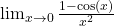
- 6.

Identify the indeterminate product form for each limit, algebraically transform the expression into a standard quotient, and evaluate using L’Hôpital’s Rule.
- 1.

- 2.

- 3.

For each of the following rational functions, use polynomial long division or the method of undetermined coefficients to determine the linear equation of the oblique asymptote.
- 1.
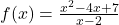
- 2.
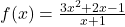
- 3.

- 4.
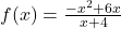
- 5.