Why do we need derivatives? In maths, we often want to understand how something is changing. For example, we might want to know how quickly a car is speeding up, how the temperature changes during the day, or how the population of a town is growing. It is not always enough to know the value of something, we also want to know how fast it is changing.
This idea of a rate of change is the motivation for derivatives. You may already know how to calculate an average rate of change, for example by looking at how much the distance travelled changes over a certain amount of time. A derivative takes this idea further: it tells us how something is changing at a particular moment. In this way, the derivative gives us information about the behaviour of a function (speed, temperature, etc.), such as whether it is increasing or decreasing and how quickly it is doing so.
Derivatives are useful in many different situations. They can help us understand motion, find maximum and minimum values, and study how different quantities are related. You do not need to think of derivatives as just a collection of rules to memorise. The important idea is that a derivative describes change. Learning about derivatives gives us a new way of looking at functions and helps us answer questions such as: How quickly is this changing? When is it increasing most rapidly? When does it reach its highest or lowest value?
The First Derivative
Imagine a car travelling along a road. Its position changes as time passes. If we take two points, and connect them with a line, the slope of that line is the average speed between those two points. The derivative of its position, at any point, tells us its speed at a particular moment. In the same way, the derivative of a function tells us how quickly its value is changing. The first derivative therefore gives us useful information about the shape and behaviour of a graph.
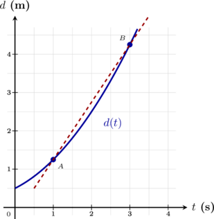
The graph of  is not a straight line. That is, at certain moments the car is driving faster than at others (covering more distance in the same time). Thus, the speed of the car changes as a function of the time. The derivative allows us to study the speed using the function .
In order to create the dashed red line that gives us the average speed we need two points. The derivative allows us to understand the instantaneous speed at any one point.
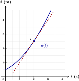
This special line, that was created using only one point and has a very specific slope is called a tangent line. We will learn more about these in our next lesson but we can already say it is tightly related to the derivative.
For now, we just need to understand what the derivative does, and how to find it. Let  be a function, its first derivative is denoted
 or
 . We use the notation with the apostrophe more commonly, but
 can also be seen.
Rules of Differentiation
In 3 periods maths, and particularly in S6, we are only concerned with finding derivatives of polynomials. Therefore, we only have a handful of rules to understand. There are four rules that concern us about derivatives, these are:
Claim (Fundamental Rules for Derivatives): Let and  be differentiable functions, and let
 ,
 , and
 be any real constants. The differentiation operator satisfies the following foundational rules:
- Derivative of a Constant: The rate of change of any fixed constant value is exactly zero:

- Constant Multiple Rule: A constant coefficient factors completely out of the differentiation process:

- The Power Rule: For any real number power , the derivative scales by the exponent and drops the variable’s power by one:

- Sum and Difference Rule: The derivative of a sum or difference equals the sum or difference of their individual derivatives:

The first and second rules should be easy to understand intuitively. If a function is constant, then the rate of change must be 0 because it does not change. Furthermore, if you look at the graph above, and we make the car at every instance twice as fast, then it makes sense that every conclusion at every point (or average of two points) is also doubled. Let us see these rules in action:
Example (Applying Differentiation Rules): Differentiate the following functions step by step, explicitly demonstrating each of the fundamental derivative rules:
 (Constant Rule)
 (Power Rule)
 (Constant Multiple Rule)
 (Sum and Difference Rule combined with all rules)
 is a fixed number that does not change with respect to

 . The
 moves to the front as a multiplier, and the exponent drops by one (
 ):

 out, then use the Power Rule on
 :





In essence, we will mostly be concerned with deriving (differentiating) polynomials, so let us see a few more examples of those.
Example (Finding the Derivative of Polynomial Functions): Find the derivative function for each of the following 4 different polynomial expressions by applying the basic rules of differentiation:



 (Expand first into a single polynomial expression)









As you can see from all of these examples, the derivative of a function is also a function. As such, it will depend on the same variable and we can replace different values of  (or
 depending on the example) to find different points belonging to the graph of the derivative. We will make more sense of why we would do this in the coming pages.
Instantaneous vs Average Rate of Change
Now we can go back to our original discussion and defined average vs instantaneous rate of change.
Definition (Rates of Change): The rate at which a variable changes relative to an independent variable can be evaluated either over an interval or at a single exact point.
1. Average Rate of Change:
The average rate of change of a function over an interval  is the ratio of the change in the output values to the change in the input values. Geometrically, it represents the slope of the line connecting the two coordinate endpoints
 and
 on the curve:

2. Instantaneous Rate of Change:
The instantaneous rate of change of a function at a point  is the average rate of change as the interval length goes to zero. Geometrically, it represents the slope of the tangent line to the curve at the point , which is also
 . That is, replace
 in :

The first definition corresponds to our first graph at the beginning of this page. The second definition corresponds to the second graph at the beginning of this page.
Example (Calculating Rates of Change): Consider the polynomial function modeling the position of an object defined by  , where represents time in seconds.
- Calculate the average rate of change of the function over the interval
 .
- Calculate the instantaneous rate of change of the function at the exact moment
 .




 . First, determine the general derivative function


 , whereas the instantaneous rate of change at the starting moment is exactly
Exercises
Find the derivative function (,  , or
 ) for each of the following 7 simple functions by applying the constant rule, the power rule, or the constant multiple rule:
Part 1: Constant Function

Part 2: Monomial Functions


Part 3: Constants Multiplied by Monomials


Find the derivative function for each of the following 6 polynomial expressions by applying the constant, power, constant multiple, and sum/difference rules:




 (Hint: Expand the expression first)
 (Hint: Expand the expression first)
The height of a model rocket in meters over time in seconds is modeled by the polynomial function  .
- Calculate the average rate of change (average velocity) of the rocket over the interval
 seconds.
- Calculate the instantaneous rate of change (instantaneous velocity) of the rocket at the exact moment
 seconds.
The total cost in Euros to manufacture hundred items at a factory is given by the function  .
- Calculate the average rate of change of the manufacturing costs over the production increase interval
 hundred units.
- Calculate the instantaneous rate of change (marginal cost) when exactly
 hundred units are produced.
The graph of a function is plotted below. The dashed red line connecting the endpoints at and  represents the average rate of change over the interval .
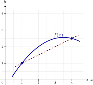
Question: For which point (value of ) on the blue curve is the instantaneous rate of change equal to the average rate of change over the interval ?
Hint: Remember that the instantaneous rate of change corresponds to the slope of a tangent line (a line touching the function only once). Use a straightedge or ruler: line it up with the dashed red secant line, and then carefully slide it across the grid while keeping it completely parallel until it intersects the blue curve only once. Identify the -coordinate where this happens.