Null Hypothesis Significance Testing

Previous Knowledge Required: Binomial Variables (S6)

Table of Contents

Motivation

Suppose a standard die is rolled 30 times and we write down the number of times the die lands on the number 6. Let $X$ be the random variable counting the number of times the die lands on 6. We know that $X\sim B(30, p)$ . You might think that $p=\frac{1}{6}$ but we do not know if the die is fair.

You would assume it is. This is what your null hypothesis (denoted $H_0$ ) will be: a generally-accepted result or assumption. In this case $H_0$ is that the die is fair, so $p=\frac{1}{6}$ . In that case, we would expect to see 5 times the number 6 (the expectation of $X$ ).

Of course, we do not always observe exactly 5 times the die landing on 6. It is going to vary or fluctuate. We know that some outcomes are more likely than others, for example, the die landing on 6 five times is more likely than it landing on 6 all 30 times. The question is, at what point is a result statistically unlikely, and at what point are our basic assumptions wrong? That is the goal of the null hypothesis significance testing (NHST).

Basic Definitions

Using our opening problem, let us say that we threw very few sixes, then we would suspect that $p<\frac{1}{6}$ . If we observed a lot of sixes, we would suspect that $p>\frac{1}{6}$ . Whichever the observed result is, it will lead to our alternative hypothesis (denoted $H_1$ ). When we do hypothesis testing, we are dealing with one of those two situations typically (having $p$ either greater or lower than a particular number). This is known as a one-tailed test. If we think that $p<\frac{1}{6}$ we are conducting a left-side/lower tail test. When we suspect $p>\frac{1}{6}$ we are conducting a right-side/upper tail test.

Say we observed the die land on 6 only once. This is our observed value. If we graph the distribution of $X$ , we see that 1 is in the lower tail. We need a measure of the amount of improbability of this particular outcome. So what is the probability of getting less than, or equal to, the observed value? That is, what is:

$P(X \le 1)$

If this probability is very small, i.e.: unlikely to happen, yet it has happened, then we are going to suspect the die is biased. This threshold is often given the symbol $\alpha$ . This is called the significance level of the test.

That particular value in most cases is $5\%$ , but could also be $10\%$ or even $1\%$ . We are setting a limit to when we are going to reject (claim it is wrong) our null hypothesis. We reject $H_0$ if the probability that we are studying is less than our significance level. That is:

$P(X\le1)<\alpha$

In the context of our problem, this means we could conclude the die is not fair. The same is true for the upper tail. If we observed a lot of sixes, we would suspect the exact same thing, just with $p>\frac{1}{6}$ . If we observed that it landed on 6 $x$ times, we would reject $H_0$ if:

$P(X \ge x) \le \alpha$

Notice how the inequality sign, comparing the probability to our significance level, is always the same!

We can either reject the null hypothesis or fail to reject the null hypothesis. An important distinction here is that we do not accept the null hypothesis, we simply disprove it or do not have enough evidence to disprove it.

If our alternative hypothesis is simply that the probability is different from the suspected value, then this requires a two-tailed test. If we take a significance level $\alpha$ , we test at half that significance level on each side of the tail.

How to Conduct a NHST

When we undertake a hypothesis test, we take the following steps:

Establish a null and alternative hypothesis, with relevant probabilities (typically stated in the
question).
Assign probabilities to our null and alternative hypotheses.
Write out our binomial distribution, assuming the null hypothesis.
Compare probability against significance level.
Draw a Conclusion – Reject or fail to reject the null hypothesis.

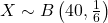
Example: A standard six-sided die used in a board game is thought to be biased because it does not roll a 1 as frequently as the other five values. In $40$ rolls, 1 appears only three times. At a $5\%$ significance level, test whether this die is biased. Let $X$ be the number of times a six-sided die was rolled, giving a result of one. Let $p$ be the probability of rolling a 1 in a roll of the die.

Another way to approach this problem is by understanding the critical values. These are the threshold values below/above which we can certainly reject the null hypothesis. In the context of our previous problem, if we rolled a 1 a total of 20 times, it would be obvious that the die is not fair and we would reject the null hypothesis. What about if we roll a 1 only 6 times? What about 9? When do we draw that line. That is the critical value.

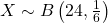
Example: Is a normal six-sided die fair when $1$ six is thrown in $24$ throws? Conduct a hypothesis test at a $5\%$ significance level.

In simpler terms, we observed a number of sixes that is relatively close to the expected number. Therefore, there is evidence to suggest the die is fair, or there is not enough evidence to suggest it is biased. We could also reason this differently. Let us find the number of times that would lead us to suspect the die is biased. That is, we want an $a$ and $b$ such that:

$\mathbb{P}(X \le a)>0.05 \quad \text{and} \quad \mathbb{P}(X \ge b)<0.05$

Here, we have $a = 0$ and $b = 8$ . That is, if we did not roll a $6$ once, or we rolled it at least $8$ times, we would suspect our die is unfair with a significance level of $10\%$ . These are called our critical values and the test we conducted in this alternative solution is a two-tailed test. We check $5\%$ on each side of the tail, so the total significance level is $10\%$ .

Example: A teacher believes that $30\%$ of students watch football on a Saturday afternoon. The teacher asks $50$ students, and $21$ of them watch football on the weekend. State at a $10\%$ level of significance whether or not the percentage of pupils that watch football on a Saturday afternoon is different from $30\%$ .

Type I and Type II Errors

These errors are statistical concepts. A type I error is a false positive, i.e.: when you incorrectly reject a true null hypothesis. A type II error is a false negative, i.e.: when you fail to reject a false null hypothesis. In short, we have:

	Reality: $H_0$ is true	Reality: $H_1$ is true
We accept $H_0$	Correct Decision	Type II error
We reject $H_0$	Type I error	Correct Decision

The process of NHST is the following, we observe (say) some $\mathbb{P}(X>x)$ . We reject the null hypothesis because the probability is lower than our significance level. To calculate the type 1 error, we calculate:

$\mathbb{P}(X>x|H_0\text{ is true})$

This is the same probability we calculated before because we were assuming our null hypothesis already.

To calculate a type II error, we find the probability of the complementary event assuming $H_1$ is correct.

Example: A quality control engineer believes that $30\%$ of electronic components produced by a factory require software firmware updates before shipping. They test a random batch of $50$ components and find that $21$ of them actually need the update. Test at a $10\%$ significance level whether the true proportion is different from $30\%$ , finding the critical values explicitly. Then, evaluate the probabilities of committing Type I and Type II errors for this quality tracking process.

Step 1: Set up the hypotheses and test criteria
Since we are testing whether the proportion is different from $30\%$ , this is a two-tailed test. We divide our $10\%$ significance level equally, placing a $5\%$ threshold ( $\alpha = 0.05$ ) in each tail. Under the null hypothesis $H_0: p = 0.3$ , the number of components requiring an update follows the distribution $X \sim B(50, 0.3)$ .

Step 2: Find the critical values and regions
Using a calculator to inspect the cumulative binomial distribution bounds for $B(50, 0.3)$ , we find the largest value $a$ and the smallest value $b$ that satisfy the $5\%$ tail criteria:

For the lower tail:

$\mathbb{P}(X \le 9) = 0.0401 \quad (< 0.05)$

$\mathbb{P}(X \le 10) = 0.0789 \quad (> 0.05)$

Therefore, the lower critical value is $9$ , and the lower rejection region is $X \le 9$ .

For the upper tail:

$\mathbb{P}(X \ge 21) = 0.0478 \quad (< 0.05)$

$\mathbb{P}(X \ge 20) = 0.0848 \quad (> 0.05)$

Therefore, the upper critical value is $21$ , and the upper rejection region is $X \ge 21$ .

The critical values are $9$ and $21$ . Since our observed value of $21$ falls inside our rejection region, we reject the null hypothesis in favour of the alternative one.

Step 3: Calculate the probability of a Type I error
A Type I error occurs if we reject the null hypothesis when it is actually true. This is exactly equal to the total probability of falling inside either rejection region under $H_0$ :

$\text{Type I Error} = 0.0879$

There is approximately an $8.8\%$ chance we incorrectly rejected the null hypothesis. This total actual error is, as expected, less than our specified $10\%$ significance level.

Step 4: Calculate the probability of a Type II error
A Type II error occurs if we fail to reject the null hypothesis when it is false. This corresponds to the probability of landing outside the critical regions (in the acceptance region $10 \le X \le 20$ ) given that the alternative hypothesis parameter is true.

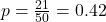We use our observed sample proportion $p = \frac{21}{50} = 0.42$ as the true alternative parameter value:

$\text{Type II Error} = \mathbb{P}(10 \le X \le 20 \mid p = 0.42)\approx0.4458$

Interpretation:
If the true proportion of components requiring updates is actually $42\%$ , there is a $44.6\%$ chance our test will fail to reject the null hypothesis. Alternatively, we can say there is a $55.4\%$ chance ( $1 - 0.446 = 0.554$ ) of correctly identifying that $p \neq 0.3$ .

Exercises

For each of the following independent scenarios, identify the population parameter of interest ( $p$ ), state the null hypothesis ( $H_0$ ) and the alternative hypothesis ( $H_1$ ) using proper statistical notation, and clarify whether a one-tailed or a two-tailed test is required.

Scenario A: A pharmaceutical company claims that $40\%$ of patients experience immediate relief from a standard cough syrup. A medical researcher suspects that a newly formulated batch has a lower success rate and tests it on a sample of patients.
Scenario B: Historical data shows that $15\%$ of online shopping carts are abandoned before completion on a retail website. The platform introduces a simplified one-click checkout system and wants to test if the abandonment rate has changed.
Scenario C: A standard seed pack states that the germination rate of wild sunflowers is $75\%$ . An organic gardener believes that using a specialized soil treatment will increase the proportion of seeds that successfully sprout.

A manufacturing plant produces precision steel bolts. Historically, the machine has a known defect rate of $8\%$ . After a software optimization update, the floor manager suspects that the proportion of defective bolts has decreased. A random sample of $50$ bolts is drawn from the production line, and exactly $1$ bolt is found to be defective.

1. State the null hypothesis ( $H_0$ ) and the alternative hypothesis ( $H_1$ ) using the population parameter $p$ .
2. Define the random variable $X$ and state its distribution under the assumption that the null hypothesis is true.
3. Use a calculator to determine the probability of this observed sample result.
4. Conduct the hypothesis test at a $5\%$ significance level ( $\alpha = 0.05$ ) and state the conclusion.
5. Conduct the hypothesis test at a $10\%$ significance level ( $\alpha = 0.10$ ) and draw the relevant conclusion.
6. Comment on why changing the significance level alters the final contextual conclusion of the test.

A magician suspects that a coin used in a theatrical performance is biased in favour of heads. To investigate this, the coin is flipped $30$ times.

1. State the null hypothesis ( $H_0$ ) and the alternative hypothesis ( $H_1$ ).
2. Assuming $H_0$ is true, define a relevant random variable $X$ and state its distribution.
3. Use a calculator to find the critical value and the corresponding rejection region for an upper-tail test at 5% significance level.
4. Suppose that exactly $22$ heads were observed during the trial. Determine whether the magician can reject the null hypothesis at this significance level.
5. If instead exactly $18$ heads had been observed, determine whether the magician could reject the null hypothesis. Justify your answer using your established critical values.

A delivery courier claims that $80\%$ of express parcels arrive before the scheduled time window. A logistics manager suspects the real success rate is lower. They track a random sample of $40$ express shipments to conduct a lower-tail test at a $5\%$ significance level ( $\alpha = 0.05$ ). Under the null hypothesis, the number of on-time arrivals follows the distribution $X \sim B(40, 0.80)$ .

1. State the null hypothesis ( $H_0$ ) and alternative hypothesis ( $H_1$ ).
2. Use a calculator to show that the critical region (rejection region) for this lower-tail test is given by $X \le 27$ .
3. Calculate the exact probability of committing a Type I error.
4. Suppose that the true underlying on-time delivery rate has actually degraded to $65\%$ ( $p = 0.65$ ). Use a calculator to determine the probability of a Type II error.