This page is dedicated to a special type of continuous random variable, those having a particular probability density function called the normal distribution. Recall that given a variable  we use the notation
 (expectation of ),
 (standard deviation), and
 (variance) is sometimes represented as
 .
Defining the Normal Distribution
Definition (Normal Distribution): A normally-distributed random variable is given by two parameters (two numerical descriptive measures), the mean  and the standard deviation
 . In this case, we say
 and the PDF is given by:
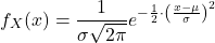
This function has the following graph, called a Bell curve:
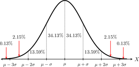
The probability density function is an adaptation of the function  . This function does not have an elementary primitive. That is, we cannot express its integral just as some simple function like we have done for polynomials or trigonometric functions.
Therefore, since it is too complicated at this level to integrate, there are two options.
- We are allowed a technological tool to calculate probabilities.
- We are asked for very specific probabilities which we know from the graph above.
When we say the first number represents the expectation and the second the variance. E.g.:  we should understand that the expectation is 0 and the standard deviation is 2 (because the variance is 4). That is:
 and
 . Some sources might use the notation
 , in which case the standard deviation would be 4, so make sure you know beforehand which notation is used in your case.
Why the Normal Distribution is so Special
The Normal Distribution is uniquely important in statistics, physics, data science, and nature primarily because of a special theorem called the Central Limit Theorem. This theorem states that if you take a large number of independent random variables and add them together, their normalised sum tends towards a normal distribution, regardless of the original distribution of the original variables.
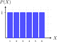
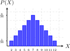
In other words, taking enough of independent variables, they begin to behave like a normal distribution. Take for example an experiment you likely have seen in previous years: Roll a dice  times and add the results. Below are the distributions for
 and
 .
1 Die Roll
2 Dice Rolls (Sum)
3 Dice Rolls (Sum)
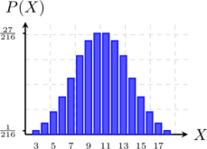
As you can see, the more dice we roll, the more the shape of the distribution resembles that of the normal distribution.
Another reason why normal variables are so important is that all the information about is given by and . Once you know these, you can draw its distribution easily.
Another interesting property of the normal distribution comes from its density function. That function is symmetric with respect to its mean. Therefore, if represents the mean of a normally-distributed random variable , then:
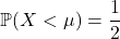
and the same for
 . That is, the mean marks what we understand as the “centre”.
Calculations with Normal Distribution
Let us see a few examples with and without calculator.
Example: A marine biology study monitors the migration weights of a specific salmon population. The data shows that their weights are normally distributed with a mean () of  and a standard deviation () of
 . Draw the distribution graph for this random variable, marking the values at
 ,
 , and
 standard deviations away from the mean alongside their precise interval percentages. Then, use the graph to calculate the probability
 .
 and
 , find the specific values on the horizontal axis:



 , applying the precise percentages dictated by the empirical rule:
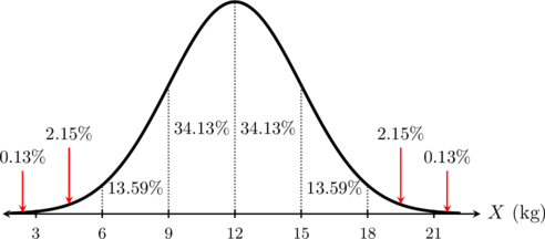
 and
 (
 to
 ):


 ):

 and
 is exactly
 (or
 ).
We could calculate this probability because it was exactly within so many standard deviations from our mean. For any other value that is not those special values, we would need a calculator. What we calculate above is that the proportion of salmon weighing between 6kg and 15kg is 81.85%.
Example: The daily charge capacity of a solar battery array at a clean energy research farm is normally distributed with a mean () of  and a standard deviation () of
 . Use a calculator to evaluate the following probabilities directly:
- 1. The probability that the array stores less than
 on a randomly selected day.
- 2. The probability that the array stores between
 and
 .
 and
 . These are not the standard values that we use our table for so we need a calculator. Your calculator should have a distribution/probability option where you can input the parameters
 and
 .
 ) in the calculator layout and input the upper bound parameter
 :

 chance that the storage capacity falls below
 ) and enter the respective limits
 and
 :

 chance that the daily storage capacity will fall between
The second the exercise gives us the mean and standard deviation, every probability can be easily found using a calculator. You may notice that at times we use  and at times
 . Remember that for a continuous random variable, we have
 (the likelihood of being an exact value is always 0) so that these two probabilities are always equal.
Understanding the Graph of the Distribution
A useful exercise to understand probabilities without a calculator is to draw the graph of the normal distribution given the mean and standard deviation.
Example: The shelf life (in days) of a particular organic dairy product is normally distributed with a mean () of  days and a standard deviation () of days.
- Complete the bell curve for this distribution using the given standard deviation benchmarks.
- What proportion of products last more than
 days?
- What proportion of products last less than
 days?
- What proportion of products last between
 and
 days?
 ) from the mean (
 ):



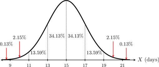
 . Summing the interval percentages to the right of this benchmark gives:

 . Summing the tail intervals to the left of this benchmark gives:

 (
 (

Normal Quantiles
By now we have found probabilities such as:  and
 . What happens when we know the probability but we want to understand the value of
 ? That is the point of normal quantiles.
We know, from the symmetry of the density function, that  . Therefore, if we are told that:
 we can conclude that 20 must be the expectation of . Similarly, we can understand other values (with or without a calculator) based on our knowledge of what the probability is.
Example: Let be a normally distributed random variable with a mean () of and an unknown standard deviation (). Given that  , determine the value of the standard deviation .
 (or
 ).

 ):



Your calculator should be able to find normal quantiles when they do not match a particular benchmark.
Example: The length of newborn sea turtles in a wildlife sanctuary is normally distributed with a mean () of  and a standard deviation () of
 . Biologists want to identify the threshold length for the smallest
 of the population to give them extra nutritional monitoring. Find the
 percentile length
 such that
 .
 ) does not correspond to an exact benchmark of

 or less to fall into the smallest
We could have guessed, based on the answer, that should be below 58 (at least one standard deviation away) but more than 54 because otherwise the probability that is left on our curve would be much less than 10%.
Exercises
The operational lifespan of a specific model of marathon running shoes is normally distributed with a mean () of  and a standard deviation () of
 . Use the empirical rule benchmarks to determine the following proportions without a calculator:
- 1. Find the probability that a pair of shoes lasts more than
 :
 .
- 2. Find the probability that a pair of shoes lasts less than
 :
 .
- 3. Find the probability that a pair of shoes lasts between
 and
 :
 .
- 4. Find the probability that a pair of shoes lasts between and :
 .
The active battery life of a new generation smartwatch on a single charge under typical usage is normally distributed with a mean () of  and a standard deviation () of
 . Apply the precise normal distribution percentages to evaluate these metrics mentally:
- 1. What proportion of smartwatches will run out of charge in under
 ? Evaluate
 .
- 2. What proportion of smartwatches will maintain a charge for over
 ? Evaluate
 .
- 3. What proportion of smartwatches will last between
 and
 ? Evaluate
 .
- 4. What proportion of smartwatches will last between and
 ? Evaluate
 .
The maximum daily flight radius of worker honeybees from an apiary during prime foraging season is normally distributed with a mean () of  and a standard deviation () of
 . Use the empirical rule to deduce the following outcomes:
- 1. Find the probability that a worker bee stays within
 of the apiary:
 .
- 2. Find the probability that a worker bee journeys further than
 :
 .
- 3. Find the probability that a worker bee travels between
 and
 :
 .
- 4. Find the probability that a worker bee travels between and
 :
 .
For each scenario below, the boundaries do not fall on exact standard deviation benchmarks. Use the calculator to evaluate the probabilities directly.
- 1. The drying time of a specific industrial eco-paint is normally distributed with a mean () of
 and a standard deviation () of
 . Find the probability that a randomly selected wall patch takes between
 and
 to dry completely:
 .
- 2. The daily water consumption of a hydroponic vertical farm house is normally distributed with a mean () of
 and a standard deviation () of
 . Find the probability that the farm house consumes more than
 on a randomly chosen day:
 .
A manufacturing process produces mechanical components whose individual weights are normally distributed with a mean () of  and a standard deviation () of
 . Draw the distribution graph for this random variable, marking the values at , , and standard deviations away from the center line alongside their precise interval percentages.
The operational runtime of an commercial LED light bulb model before burning out is normally distributed with a mean () of  and a standard deviation () of
 . Construct the symmetrical bell curve for this distribution system, clearly labeling the horizontal axis axis increments for
 ,
 , and
 .
For each scenario below, use the given parameters to compute the specified interval probabilities and find the requested normal quantile threshold value using a statistical calculator or distribution table.
- 1. The score on a national professional licensing exam is normally distributed with a mean () of
 points and a standard deviation () of
 points.
a. Find the probability that a randomly chosen candidate scores between and
 points:
 .
b. Find the minimum passing score required to be in the top of candidates (the
 percentile threshold value such that
 ).
- 2. The volume of juice bottled by an automated manufacturing machine is normally distributed with a mean () of
 and a standard deviation () of
 .
a. Find the probability that a randomly selected bottle contains less than :
 .
b. Determine the maximum volume threshold for the bottom under-filled bottles (the
 percentile threshold value such that
 ).
Let be a normally distributed random variable modeling a manufacturing or natural scenario. Use your knowledge of the empirical rule benchmark percentages to deduce the standard deviation for the following problem:
- A normally distributed random variable has an expectation () of
 . Knowing that the probability of falling between
 and
 is exactly
 (
 ), determine what the standard deviation must be.