In this page we do a small revision of the most famous models you have seen in S4-S5 while also discussing two new concepts from analysis, namely: domain and range.
A lot of this should be mostly a reminder, but the understanding should be very clear to better grasp future concepts.
Domain and Range
We begin with the definitions, then we clarify them:
Definition (Domain): The domain of a function  is the set of all possible values (typically represented by the variable
 ) for which the function is defined and gives an output.
Geometrically, if you look at the graph of a function, the domain corresponds to the horizontal shadow or projection of the entire curve onto the -axis.
Polynomials (which you have seen in S4) are defined everywhere. Therefore, if  is a polynomial, the domain of is:

 or
 to say that every real number can be replaced. This includes linear models, quadratic models, cubic models, and for any other polynomial.
So when is the domain not every real number? A simple example from S4 is an inverse proportion model:
Example: Determine the domain for each of the following rational functions:





 . In interval notation, this domain is written as:

As you can see, as soon as we have a fraction, the domain will be any value of that would make the denominator zero. The domain could also exclude an entire collection of numbers. For example:
Example: Determine the domain for each of the following radical functions:



![\[[0, \infty)\]](https://mathematics.lu/wp-content/ql-cache/quicklatex.com-ebdab0c268faf630141ef98b351d2438_l3.png "Rendered by QuickLaTeX.com")


 . In interval notation, this domain is written as:
![\[[2, \infty)\]](https://mathematics.lu/wp-content/ql-cache/quicklatex.com-020a0d16e5cb4168aea9df71a9ea9dc4_l3.png "Rendered by QuickLaTeX.com")
Typically, we will look at functions and instantly understand what values of could be “problematic”.
The logarithmic function  , which you will see in S7, has 3 different rules that define its domain:


Again, this is a function you will explore in S7. For now, we move on to our next definition.
Definition (Range): The range of a function is the set of all output values (typically represented by the variable  ) that the function generates when you plug in every valid value from the domain.
Geometrically, if you look at the graph of a function, the range corresponds to the vertical shadow or projection of the entire curve onto the -axis, tracking from the absolute lowest point to the absolute highest point.
This one is harder to understand algebraically. The proper way to do it would be by looking at the domain of its inverse. However, this is not something covered in the programme, so you are just expected to recognise domain and range by looking at the graph of a function.
Given the graph of a function , suppose there are two flashlights on the sides (left and right). The portion of the -axis covered by the shadow is the range of . Similarly, if we had two flashlights above and below the graph, the portion of the -axis covered by the shadow of the graph is the domain.
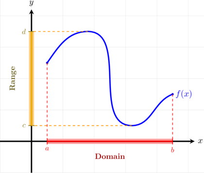
For some functions, the range may be easier to find. For example, you learned in S5 that parabolas have a vertex. This vertex will represent either a maximum or minimum of your function, so you know exactly where the highest/lowest point of your range is.
Axes Intercepts
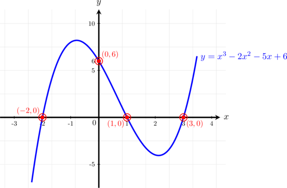
These are easy to recognise on the graph, but we still need a way to understand them formally. We have the -intercept(s) (could be more than one) and the -intercept.
To find the -intercepts of a function , we solve the equation  . The values that solve that equation are the -intercepts. To find the -intercept of a function , we calculate
 (assuming
 is in the domain of ). The answer is the -intercept.
Example: Find the coordinates of all axis intercepts for the quadratic function defined by:


 .




 and
 .
Not every function necessarily has either intercept. If a function has a -intercept, it can only have 1. You may recall from S4 the vertical line test. Were a function to have more than one -intercept, the -axis would be a vertical line that intersects the graph more than once, so it would not qualify as a function.
A function could have infinite -intercepts, as you must have seen in S5 when discussing trigonometric functions and periodic models.
In short, we have:
A function with neither intercept is  . This is because the fraction will never equal zero, as the numerator is fixed. On the other hand, we cannot replace
 because we cannot divide by 0. Therefore, it has neither intercept.
Linear Models
We begin with a definition:
Definition (Linear Models): An algebraic function that models a constant rate of change between an independent variable and a dependent variable, representing a straight line on a graph.

 : The slope, which measures the steepness and direction of the line as a constant rate of change.
 : The y-intercept, representing the initial value where the straight line crosses the vertical y-axis.
If  , then the more increases, the more increases. If
 , the more increases, the more decreases. The slope can be calculated as:

 and
 , the slope of the line connecting them is:

 to find the value of , since we’d know 3 out of the 4 elements in that equation. Let us see an example of this:
Example: Find the equation of the straight line that passes through the two points  and
 in the form
 .
 and
 :

 and the coordinates of the first point


Two special cases of linear models are vertical and horizontal lines. Horizontal lines have a constant , so their equation is  with
 . Vertical lines are lines of the form
 with a constant.
Linear models are an example of polynomials. In fact, they are polynomials of degree 1. All polynomials are continuous functions (an idea that is not fully studied in the programme, but we will get back to this in due time). They are defined everywhere, so lines are defined everywhere.
With the exception of horizontal lines, the range of any linear function is .
Quadratic Models
Definition (Quadratic Models): An algebraic function containing a second-degree polynomial variable that models non-linear relationships, producing a symmetric, U-shaped curve known as a parabola when graphed.

 : The leading coefficient, which determines the vertical scaling and the direction the parabola opens (upwards if positive, downwards if negative).
 : The linear coefficient, which influences the horizontal and vertical position of the parabola’s vertex alongside .
 : The constant term, representing the exact y-intercept where the curve intersects the vertical axis.
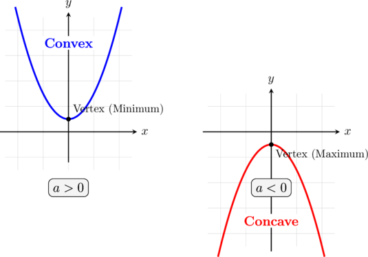
Quadratic models are polynomials of degree 2. As such, they are defined everywhere. They have a special point called the vertex which represents its lowest/highest point depending on the value of . If  , the vertex is a minimum. If
 the vertex is a maximum. This idea we will generalise when we get to the analysis unit.
The vertex of the parabola has -coordinate given by  . The -coordinate of the vertex is given by
 (replacing
 into the equation of your function).
Example: Find the coordinates of the vertex for the quadratic function  and determine whether it represents a maximum or minimum point using the leading coefficient.
 and
 , then apply the vertex formula:



Since the vertex represents a maximum or minimum, understanding the range of a parabola is actually rather easy. If the parabola has a maximum at  , then the range is
![(-\infty,y_v]](https://mathematics.lu/wp-content/ql-cache/quicklatex.com-4966e69cca8ddc75c059705de2dbf2bc_l3.png "Rendered by QuickLaTeX.com") . If it has a minimum, the range is
 .
We clarify that we take  to mean the interval of all points
 between and not including the endpoints and
 to be all the points including and .
We have already discussed how to find the axes intercepts of functions, but we just remind that a quadratic equation of the form  can be solved using the quadratic formula:
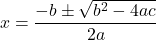
 is denoted
 and called the discriminant. Depending on its value, the number of real solutions the equation has:
- If
 , the equation has two real solutions.
- If
 , the equation has exactly one solution.
- If
 , the equation has no real solutions. Since we saw complex numbers, we know now that there are 2 complex solutions in this case.
We mentioned the role of the parameter in the quadratic model  by determining which way the parabola will face. The words happy or sad sometimes refer to the type of parabola ( being happy and being sad). In reality, we call these convex and concave respectively. These two words will take a higher meaning in the analysis unit.
Inverse Proportionality Models
These are functions of the form  with
 some constant. They describe an inverse proportion between the -variable and the -variable, i.e.: if is doubled, is halved, and so on.
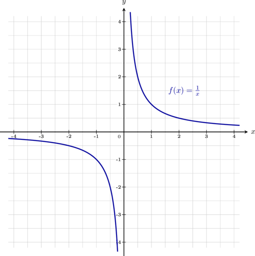
Whenever we have a function that is defined with a fraction, the denominator must be different from zero. Otherwise, the function is not defined. That is, the domain of an inverse proportionality model will never include , as we can see on the graph of .
We can also study functions where small changes are made to either the numerator or denominator.
Example: Find the domain of the rational function defined by:
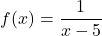
State your final answer in set notation and interval notation.


 , the denominator becomes zero, forcing the entire function to be undefined at that point.
 :


We can also find axes intercepts when both numerator and denominator are linear functions. This is no longer an inverse proportionality model, but it is a good exercise to practice some basic algebra. Even though this example is somewhat above the 3-period level, you can see that there is nothing special to it.
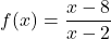
Example: Find the coordinates of both the -intercept and the -intercept for the rational function defined by:
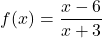


 , the denominator is
 , which is perfectly valid. Written as a coordinate pair, the
 .


 .
Exponential Models
In S5, you discussed exponential functions and modelled situations of exponential growth and decay.
Definition (Exponential Model): An exponential model is a mathematical function used to model scenarios where a quantity changes at a rate proportional to its current value. The standard base- exponential function is expressed in the form:

Core Parameters and Parameters Analysis:
- Initial Population (
 ): The constant coefficient represents the initial value or starting population of the system. This is because evaluating the function at
 yields:

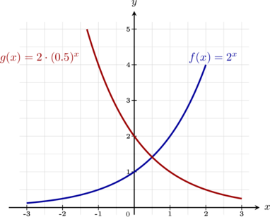
- Exponential Growth (
 ): If the base is strictly greater than
 , the function models exponential growth. As increases, the output values grow larger at an accelerating rate (e.g., compounding interest or bacterial growth).
- Exponential Decay (
 ): If the base is a fraction between and , the function models exponential decay. As increases, the output values decrease toward zero at a decelerating rate (e.g., radioactive decay or drug clearance in a bloodstream).
The domain of these functions is , that is, we can replace any . The range is typically all the positive or all the negative numbers, depending on the value of . The exponential function is never zero, so these functions will never intersect the -axis unless they are modified or subtracted a constant value. Therefore, they are either always above ( ) or always below (
 ) the -axis. Since we typically use these to model populations, they will likely be positive, but you could also model temperature changes in a room, in which case it could definitely be negative.
You also solved word problems related to exponential growth and decay.
Example (Exponential Growth): A population of bacteria in a petri dish is modeled by the function  , where
 is the time measured in hours and
 is the total number of bacteria.
- Identify the initial population and calculate the percentage growth rate per hour.
- Determine the bacteria population at times
 ,
 , and
 hours.
 , where
 and the growth factor is
 .
 , this represents exponential growth. We express the growth factor as
 , where
 is the growth rate:

 .
 :



To finish our reminder, we see an example of exponential decay.
Example (Exponential Decay): The mass of a radioactive substance left in a laboratory sample is modeled by the function  , where is measured in days and
 is the remaining mass in grams.
- Identify the initial mass and calculate the percentage decay rate per day.
- Determine the remaining mass of the sample at times , , and days.
 and the decay factor is
 .
 , this represents exponential decay. We express the decay factor as
 , where

 .



Exercises
Determine the domain of each of the functions below. Express each domain using interval notation. State any restriction rules applied, such as avoiding division by zero or negative values under square roots.

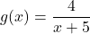
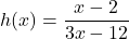
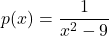

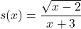
For each of the following functions, calculate the coordinates of all x-intercepts and y-intercepts. Remember to state your final answers as coordinate pairs  .




For each pair of coordinate points below, determine the algebraic equation of the straight line passing through them. Express each final answer in standard gradient-intercept form, .
 and

 and

 and

 and

 and

 and

For each of the following four quadratic functions, calculate the exact coordinates of the vertex. Then, classify whether the vertex is a maximum or minimum point by analysing the leading coefficient.




For each of the following three quadratic functions, find the coordinates of all axes intercepts. Calculate the exact -intercept by evaluating , and find any real -intercepts by solving  .
