In S6, you learned about discrete random variables, variables that are typically the result of counting. Continuous random variables are those that result from measuring. For example, we can measure heights, weights, time elapsed.
Motivation
Consider the following situation: You are playing darts and you have the following board:
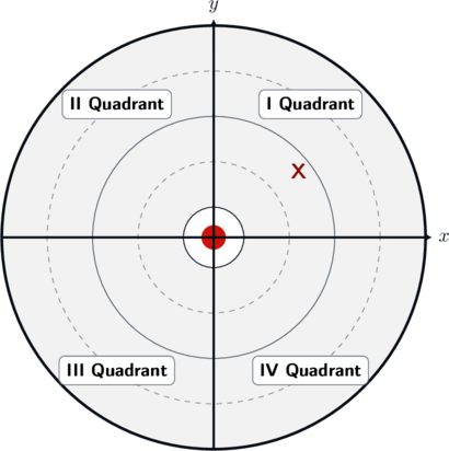
What is the likelihood that if you throw a dart, it lands on the 2nd quadrant? The correct and even intuitive answer would be  . Why is that? Simply put, the 2nd quadrant occupies a quarter of the circle (of the entire board) and so the likelihood of a dart landing there is . This logic is perfectly correct. What we are comparing is areas. This is how we calculate probabilities with continuous random variables.
The next example is a bit trickier. What is the likelihood that the dart lands exactly on the X? The answer is 0. Think of it in terms of how many points there are on the board. You want 1 precise point out of infinite points. Therefore, it makes sense that this probability is 0.
Even with our area comparison, the area of a point is 0, so the probability should also be zero. A small side-discussion could be: if you can say this about any point, then it would make sense that a dart can never land on the board. This is not true because there are infinite points, and our logic breaks down when we try to expand a finite situation into infinity.
This is the same logical problem as when we compare  with
 (periodic).
Definitions
In this section, we define how to find probabilities of a continuous random variable and also extend the concepts we saw for discrete random variables (i.e.: expectation, variance, and standard deviation) to continuous random variables.
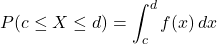
Definition (Probability Density Function – PDF): A Probability Density Function  is a function that describes the probability for a continuous random variable
 to take on certain values. is defined on some interval
 . The probability that falls within a specific interval
 is given by the integral of the PDF over that interval:
Conditions for a Valid PDF: For to be a valid probability distribution function, it must satisfy the following two properties:
- 1. Non-negativity: The function cannot have negative values:

- 2. Total Probability: The total area under the entire curve must equal exactly :
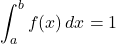
In other words, we have an image like this to calculate  .
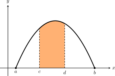
This also explains why the probability of being an exact value is always 0.
Example: Consider a continuous random variable with the probability density function given by  for
 . Verify that is a valid probability density function, and then calculate the probability
 .
 is always greater than or equal to zero. We can see this by looking at the graph of the function (or using our knowledge from S5).
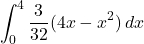






 is exactly
 .
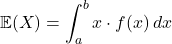
Definition (Expectation / Expected Value): The expected value (or mean)  of a continuous random variable with a probability density function , defined on , is given by:
Example: Let be a continuous random variable with the probability density function given by  defined on the interval
 , and
 everywhere else. Show that is a valid probability density function, find the probability
 , and find the expected value .
 ,
 , which implies
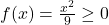 . Outside this interval,
 for all
 .
 to
 must equal exactly



 by the density function over the interval


Definition (Variance): The variance  (also denoted
 ) of a continuous random variable defined on a bounded interval with a probability density function defined on
 is given by:

The symbol  is just another way to write . This definition should be relatively intuitive. It is the same definition as you saw in the discrete case, but since we have infinite values we have an infinite sum, which is equivalent to an integral.
Definition (Standard Deviation): The standard deviation  of a continuous random variable defined on a bounded interval is the positive square root of its variance, quantifying the average spread of the probability distribution in the same units as the random variable itself.

Example: Let be a continuous random variable with a probability density function given by  defined on the interval
 . Show that is a valid probability density function, and find the expected value , the variance , and the standard deviation .
 , we have that:
 .
 must equal exactly



 over the interval


 :


Exercises
For each function below defined on a bounded interval , determine whether it represents a valid PDF.
- 1.
 defined on
 , and otherwise.
- 2.
 defined on , and otherwise.
- 3.
 defined on
 , and otherwise.
Let be a continuous random variable with the probability density function given by  defined on the bounded interval , and otherwise. Evaluate the distribution by solving the following sub-problems:
- 1. Calculate the interval probability
 .
- 2. Compute the expected value .
- 3. Find the variance
 .
- 4. Determine the standard deviation .
For each probability density function below defined on its respective bounded interval , calculate the expectation , the variance , and the standard deviation . Assume everywhere else.
- 1.
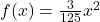 defined on the interval
 .
- 2. defined on the interval .
- 3.
 defined on the interval .
- 4.
 defined on the interval .
- 5. defined on the interval .